POMDPs II:
Electric Boogaloo
Outline
- Character development flashback: Alpha Vectors
- Approximations
- When is it actually worth it to attempt to solve a POMDP?
POMDP Sense-Plan-Act Loop
Environment
Belief Updater
Policy/Planner
\(h_t = (b_0, a_1, o_1 \ldots a_{t-1}, o_{t-1})\)
\(a\)
\[b_t(s) = P\left(s_t = s \mid h_t \right)\]

True State
\(s = 7\)
Observation \(o = -0.21\)
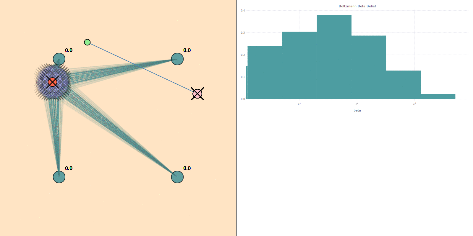
Alpha Vectors
BOARD
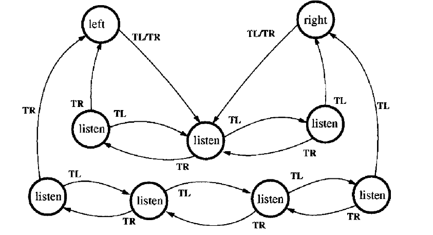
Finite State Machine Policies
Approximations
- Numerical
- Policy information restriction
- Formulation
Numerical Approximations
DESPOT, POMCP, SARSOP, POMCPOW, others
Online, Offline
Goal is to solve the full POMDP approximately
Can find useful approximate solutions to large problems IN REAL TIME
Numerical Approximations
Focus on smaller reachable part of belief space

Policy information restriction
- Certainty equivalent: \(\pi(b) = \pi_s\left(\underset{s\sim b}{E}[s]\right)\)
- Last \(k\) observations

Formulation Approximations
- QMDP
- Fast Informed Bound
- Hindsight Optimization
- Ignore Observations
- Most Likely Observation
- Open Loop
QMDP
POMDP:
QMDP:
\[\pi_{Q_\text{MDP}}(b) = \underset{a\in\mathcal{A}}{\text{argmax}} \underset{s\sim b}{E}\left[Q_\text{MDP}(s,a)\right]\]
where \(Q_\text{MDP}\) are the optimal \(Q\) values for the fully observable MDP. \(O(T |S|^2|A|)\)
$$\pi^* = \underset{\pi: \mathcal{B} \to \mathcal{A}}{\mathop{\text{argmax}}} \, E\left[\sum_{t=0}^{\infty} \gamma^t R(s_t, \pi(b_t)) \right]$$
QMDP
INDUSTRIAL GRADE
QMDP


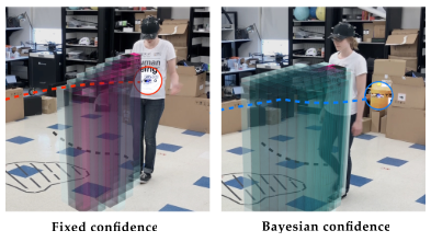
ACAS X
[Kochenderfer, 2011]
POMDP Solution
QMDP


Same as full observability on the next step
FIB (Fast Informed Bound)

\[\pi_\text{FIB}(b) = \underset{a \in \mathcal{A}}{\text{argmax}}\, \alpha_a^T b\]
- (Sort of) like taking the first observation into account.
- Strictly better value function approximation than QMDP
- \(O(T |S|^2|A||O|)\)
Hindsight Optimization
POMDP:
Hindsight:
$$V_\text{hs}(b) = \underset{s_0 \sim b}{E}\left[\max_{a_t}\sum_{t=0}^{\infty} \gamma^t R(s_t, a_t) \right]$$
$$\pi^* = \underset{\pi: \mathcal{B} \to \mathcal{A}}{\mathop{\text{argmax}}} \, E\left[\sum_{t=0}^{\infty} \gamma^t R(s_t, \pi(b_t)) \right]$$
\pi_\text{hs}(b) = \underset{a \in \mathcal{A}}{\text{argmax}} \underset{s_0 \sim b}{E}\left[R(s_0, a) + \max_{a_t}\sum_{t=1}^{\infty} \gamma^t R(s_t, a_t) \right]
Ignore Observations
Most Likely Observation
- Replace observation model with most likely given the belief or history
Open Loop
When to try the full POMDP
- Costly Information Gathering
- Long-lived uncertainty, consequential actions, and good models
- For comparison with approximations
BOARD
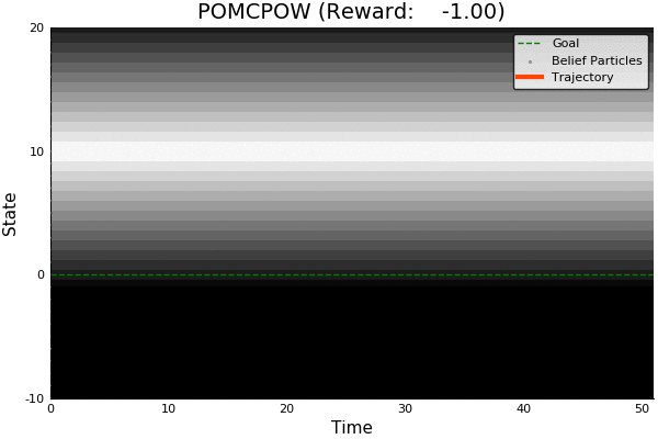
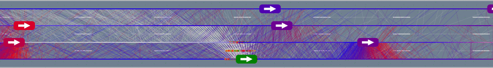
Information Gathering

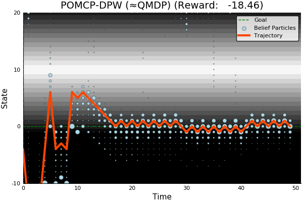
QMDP
Full POMDP


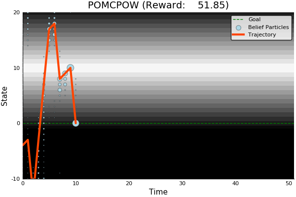

Ours
Suboptimal
State of the Art
Discretized
[Ye, 2017] [Sunberg, 2018]


Information Gathering
Costly
R(s, a) = \begin{cases}
100 & \text{ if } a = 0, s = 0 \\
-100 & \text{ if } a = 0, s \neq 0 \\
-1 & \text{ otherwise}
\end{cases}
Long-lived uncertainty
Long-lived Uncertainty
- Learnable partially observed state
- Consequential decisions
- Accurate-enough model
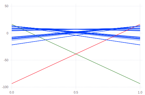
Comparison with Approximations
Comparison with Approximations
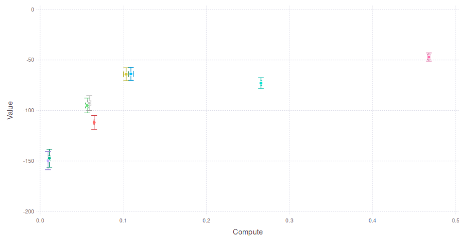
COMPUTE
Expected Cumulative Reward
Full POMDP (POMCPOW)
No Observations
POMDPs II
By Zachary Sunberg


