Dynamic

Programming

What is Dynamic Programming?

Dynamic programming Is a method for solving complex problems by breaking them down into simpler subproblems.

a DP problem usually can be solved optimally by breaking it into sub-problems and then recursively finding the optimal solutions to the sub-problems

Dynamic Programming

VS Recursion

Both are using sub-problems to solve the main problem
Recursion is much more general
If it can be solved by dynamic programming, DP is much faster
Usually DP requires more space
SPACE VS TIME

When we use DP?

Recursion is making some redundant computation
Optimal sub-structures:
optimal solutions to the original problem contains optimal solutions to sub-problems

How to use DP?

Think about the recursion solution
Find sub problems that have been computed multiple times
See if the sub problems are optimal sub-structure
Try to memorize them to avoid the redundant computing

Fibonacci Numbers

def fibonacci(n):
    if n in (0, 1):
        return 1
    return fibonacci(n - 1) + fibonacci(n - 2)

F(6)

F(5)

F(4)

F(3)

F(2)

F(1)

F(0)

F(1)

F(0)

F(1)

F(0)

F(1)

F(0)

F(2)

F(1)

F(0)

F(2)

Need some space to avoid the computation

We use an Array to store the temp result

What is the optimal sub-structure?

def fibonacci(n):
    if n <= 1:
        return 1
    result = [0] * (n + 1)
    result[0] = 1
    result[1] = 1
    for i in range(2, n + 1):
        result[i] = result[i - 1] + result[i - 2]
    return result[n]

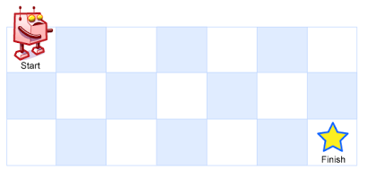
Unique Paths

Where is the redundancy?

What is the optimal sub-structure?

def uniquePaths(m, n):
    if m == 1 or n == 1:
        return 1
    return uniquePaths(m - 1, n) + uniquePaths(m, n - 1)

Unique Paths

Optimal Sub-structure

a(i,j) = a(i-1,j) + a(i, j-1)

Unique Paths

def unique_paths(m, n):
    # Initialize a 2D grid with dimensions m x n, filled with 0
    dp = [[0] * n for _ in range(m)]
    
    # Set the first row and first column to 1 (base cases)
    for i in range(m):
        dp[i][0] = 1
    for j in range(n):
        dp[0][j] = 1
    
    # Fill the rest of the grid using the recurrence relation:
    # dp[i][j] = dp[i-1][j] + dp[i][j-1]
    for i in range(1, m):
        for j in range(1, n):
            dp[i][j] = dp[i - 1][j] + dp[i][j - 1]
    
    # Return the value in the bottom-right corner
    return dp[m - 1][n - 1]

Minimum Path Sum

1	3	4	2
3	5	2	3
2	1	2	3
2	2	4	2

Best optimal sub-structure?

Given a grid filled with non-negative numbers, find a path from top left to bottom right, which minimizes the sum of all numbers along its path.

Note: You can only move either down or right at any point in time.

Minimum Path Sum

1	3	4	2
3	5	2	3
2	1	2	3
2	2	4	2

PathSum(m,n) = MIN(PathSum(m,n - 1), PathSum(m - 1,n)) + matrix(m,n)

Minimum Path Sum

def minPathSum(grid):
    if not grid or not grid[0]:
        return 0

    m, n = len(grid), len(grid[0])
    dp = [[0] * n for _ in range(m)]
    dp[0][0] = grid[0][0]

    # Initialize first row
    for j in range(1, n):
        dp[0][j] = dp[0][j - 1] + grid[0][j]

    # Initialize first column
    for i in range(1, m):
        dp[i][0] = dp[i - 1][0] + grid[i][0]

    # Fill in the rest of the table
    for i in range(1, m):
        for j in range(1, n):
            dp[i][j] = min(dp[i - 1][j], dp[i][j - 1]) + grid[i][j]

    return dp[-1][-1]

Minimum Path Sum

Any improvement?

We can use less space to get the same result without hurting time complexity

Minimum Path Sum II

def min_path_sum(grid):
    """
    Calculate the minimum path sum from the top-left to the bottom-right corner of a grid,
    where movement is only allowed to the right or down.

    :param grid: 2D list representing the grid with non-negative integers
    :return: The minimum path sum
    """
    if not grid or len(grid) == 0:
        return 0

    m, n = len(grid), len(grid[0])

    # Initialize arrays for the current and previous rows
    current_row = [0] * n
    previous_row = [0] * n

    # Initialize the first row
    previous_row[0] = grid[0][0]
    for j in range(1, n):
        previous_row[j] = previous_row[j - 1] + grid[0][j]

    # Compute the minimum path sums for the rest of the grid
    for i in range(1, m):
        current_row[0] = grid[i][0] + previous_row[0]
        for j in range(1, n):
            # Take the minimum path sum between the top and left cells
            current_row[j] = min(previous_row[j], current_row[j - 1]) + grid[i][j]
        # Update previous_row for the next iteration
        previous_row = current_row[:]

    # The last element in the final row contains the result
    return previous_row[-1]

0-1 Knapsack

Given a knapsack which can hold w pounds of items, and a set of items with weight w1, w2, ... wn. Each item has its value s1,s2,...,sn. Try to select the items that could put in knapsack and contains most value.

What is the optimal sub-structure?

0-1 Knapsack

w[i][j]: for the previous total i items, the max value it can have for capacity j

Which two we need to use to compare?

w[i][j]: for the previous total i items, the max value it can have for capacity j

When you iterate i, and j, you need to try:

If the new i could be added into j
if it could and added, could it be better

	1	2	3	4	5	6	7
0	0	0	0	0	0	0	0
1	3	3	3	3	3	3	3
2	3	3	8	11	11	11	11
3	3	3	8	11	11	11	12
4	3	3	8	11	11	11	12

w[i][j]: for the previous total i items, the max value it can have for capacity j

Example: weights{1,3,4,5} values{3,8,4,7}

def knapsack(capacity, weights, values):
    length = len(weights)
    if capacity == 0 or length == 0:
        return 0
    w = [[0] * (capacity + 1) for _ in range(length + 1)]
    for i in range(1, length + 1):
        index = i - 1
        for j in range(1, capacity + 1):
            if j < weights[index]:
                w[i][j] = w[i - 1][j]
            elif w[i - 1][j - weights[index]] + values[index] > w[i - 1][j]:
                w[i][j] = w[i - 1][j - weights[index]] + values[index]
            else:
                w[i][j] = w[i - 1][j]
    return w[length][capacity]

Coin Change

We mentioned this question in DFS and use DFS will be TLE, even with the Greedy idea.

The question is similar to knapsack

coin and amount will be the two dimension

How we update the result?

def coinChange(coins, amount):
    # Sort coins for predictable order (not essential but can help logic clarity)
    coins.sort()
    length = len(coins)

    # Initialize a 2D DP table: dp[i][j] = min coins to make amount j using first i+1 coin types
    dp = [[0] * (amount + 1) for _ in range(length)]

    # Initialize first row using only the smallest coin (coins[0])
    for j in range(amount + 1):
        if j % coins[0] == 0:
            dp[0][j] = j // coins[0]
        else:
            dp[0][j] = -1  # Not possible to form j with only coins[0]

    # Fill in the DP table for the rest of the coin types
    for i in range(1, length):
        for j in range(amount + 1):
            if j < coins[i]:
                # Can't use coin[i], so take the value from the previous row
                dp[i][j] = dp[i - 1][j]
            else:
                min_coins = float('inf')

                # Try using 0 to (j // coins[i]) of coins[i]
                for k in range(j // coins[i] + 1):
                    remaining = j - coins[i] * k
                    if dp[i - 1][remaining] != -1:
                        min_coins = min(min_coins, dp[i - 1][remaining] + k)

                dp[i][j] = min_coins if min_coins != float('inf') else -1

    # Result is the minimum number of coins to make 'amount' using all coin types
    return dp[-1][amount]

Dynamic Programming VS Greedy

Greedy algorithm: an algorithmic paradigm that builds up a solution piece by piece, always choosing the next piece that offers the most obvious and immediate benefit. So the problems where choosing locally optimal also leads to a global solution are best fit for Greedy.

Dynamic Programming VS Greedy

Dynamic programming: it's mainly an optimization over plain recursion. Wherever we see a recursive solution that has repeated calls for the same inputs, we can optimize it using DP. The idea is to simply store the results of subproblems so that we do not have to re-compute them when needed later. This simple optimization reduces time complexities from exponential to polynomial.

Algorithm relationships

Brute Force Search (DFS/Backtrace) <= For each stage, the optimal state is defined all prior stage states.
Greedy <= For each stage, the optimal state is defined by optimal state from prior stage.
Dynamic programing <= For each stage, the optimal state is defined by states from some stages, and won't care about how those states are created. (每个阶段的最优状态可以从之前某个阶段的某个或某些状态直接得到，而不管之前这个状态是如何得到的)

How to solve DP problem

Steps to solve a DP:

Identify if it is a DP problem
Decide a state expression (with least parameters)
Create state transition function
Find the boundary and build the dp table

Longest Increasing Subsequence

3, 1, 4, 5, 7, 6, 8, 2

1, 4, 5, 6, 8 (Or 1, 4, 5, 7, 8)

Longest Increasing Subsequence

What is the optimal sub-structure?

Longest Increasing Subsequence

We store lis[i] for the LIS by i?

We store lis[i] for the LIS end with sequence[i]

Longest Increasing Subsequence

  public int lengthOfLIS(int[] nums) {
        if (nums == null || nums.length == 0) {
            return 0;
        }
        
        int n = nums.length;
        int[] dp = new int[n];
        
        // Initialize dp array with 1, since the length of the LIS at each element is at least 1
        for (int i = 0; i < n; i++) {
            dp[i] = 1;
        }
        
        // Iterate through the array to find the longest increasing subsequence
        for (int i = 0; i < n; i++) {
            for (int j = 0; j < i; j++) {
                if (nums[i] > nums[j]) {
                    dp[i] = Math.max(dp[i], dp[j] + 1);
                }
            }
        }
        
        // Find the maximum value in dp array, which will be the length of the LIS
        int maxLength = 0;
        for (int i = 0; i < n; i++) {
            maxLength = Math.max(maxLength, dp[i]);
        }
        
        return maxLength;
    }

站在i的位置向之前看

看看之前的 j，寻找更长subsequence

Longest Increasing Subsequence

def longestIncreasingSubsequence(nums):
    if not nums:
        return 0
    
    n = len(nums)
    dp = [1] * n
    
    # Iterate through the array to find the longest increasing subsequence
    for i in range(n):
        for j in range(i):
            if nums[i] > nums[j]:
                dp[i] = max(dp[i], dp[j] + 1)
    
    # Return the maximum value in dp array, which is the length of the LIS
    return max(dp)

State mathematical description

Given a series of numbers of size N,

Assume F(k): the LIS length, which end with kth number in the series.

Q: Find the max in F(1)...F(N)

Longest Common Sequence

Example: abcfbc abfcab

return 4 (abcb)

Longest Common Sequence

Example: abcfbc abfcab

return 4 (abcb)

Longest Common Sequence

What is the optimal sub-structure?

maxCommon(i,j): longest common string for String A(0,i) and String B(0,j)

We finally need to get maxCommon(stringA.length, stringB.length)

Longest Common Sequence

What is the relationship between maxCommon(i,j) and maxCommon(i-1,j-1)?

If(A[i-1] = B[j-1]) ?

If(A[i-1] != B[j-1])?

Longest Common Sequence

What is the relationship between maxCommon(i,j) and maxCommon(i-1,j-1)?

If(A[i-1] = B[j-1]) ?

If(A[i-1] != B[j-1])?

maxCommon(i,j) = maxCommon(i-1,j-1) + 1

maxCommon(i,j) = max(maxCommon(i-1,j), maxCommon(i,j-1))

Longest Common Sequence

def longestCommonString(a, b):
    m = len(a)
    n = len(b)
    maxCommon = [[0] * (n+1) for _ in range(m+1)]
    for i in range(1, m+1):
        for j in range(1, n+1):
            if a[i-1] == b[j-1]:
                maxCommon[i][j] = maxCommon[i-1][j-1] + 1
            else:
                maxCommon[i][j] = max(maxCommon[i][j-1], maxCommon[i-1][j])
    return maxCommon[m][n]