A High-Performance Ocean Simulator in Pure Python
Dion Häfner
AMS 98th Annual Meeting
Photo: Jong Marshes on Unsplash
Veros

TL;DR: The versatile ocean simulator.
Vision:
- Accessible: Easy to get started
- Scalable: Runs on your laptop, gaming PC, or cluster
- Verifiable: Readable code, minimal boilerplate
- Powerful: No compromises on functionality
- Adaptable
Ocean modeling made fun
Implementation:
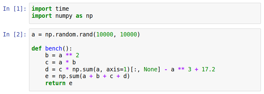
- Direct translation of pyOM2's Fortran backend to NumPy
- Pythonic frontend & config
- Some linear algebra, mostly number crunching
- I/O through netCDF4 & HDF5
What is ?
PyOM2
Features:
- Solves full 3D primitive equations on C-grid (spherical or pseudo-Cartesian)
- Several parameterizations for diffusion, friction, advection, EKE, TKE, IW, isoneutral mixing, EOS, ...
- Pre-configured idealized and realistical configurations
Implementation:
- Numerical routines in Fortran
- Configuration in Python (f2py) or Fortran
- Parallelized via MPI
- I/O via netCDF4
Grand total: 18,000 SLOC
An ocean model by Carsten Eden (Hamburg University)
Fortran to NumPy
do j=js_pe,je_pe
	do i=is_pe-1,ie_pe
		flux_east(i,j,:) = &
			0.25*(u(i,j,:,tau)+u(i+1,j,:,tau)) &
			    *(utr(i+1,j,:)+utr(i,j,:))
	enddo
enddo
vs.flux_east[1:-2, 2:-2,:] = \
0.25 * (vs.u[1:-2, 2:-2, :, vs.tau] + vs.u[2:-1, 2:-2, :, vs.tau]) \
* (vs.utr[1:-2, 2:-2, :] + vs.utr[1:-2, 2:-2, :])Fortran to NumPy
yt(1)=yu(1)-dyt(1)*0.5
do i=2,n
yt(i) = 2*yu(i-1) - yt(i-1)
enddoyt[0] = yu[0] - dyt[0] * 0.5
yt[1:] = 2 * yu[:-1]
alternating_pattern = np.ones_like(yt)
alternating_pattern[::2] = -1
yt[...] = alternating_pattern * np.cumsum(alternating_pattern * yt)Fortran to NumPy
- Convert conditions in loops to masks
- Broadcasting via newaxis
- Let's avoid fancy indexing
ks = vs.kbot[2:-2, 2:-2] - 1
ki = np.arange(vs.nz)[np.newaxis, np.newaxis, :]
boundary_mask = (ks >= 0) & (ks < vs.nz - 1)
full_mask = boundary_mask[:, :, np.newaxis] & (ki == ks[:, :, np.newaxis])
vs.eke_lee_flux[2:-2, 2:-2] = np.where(
boundary_mask,
np.sum(vs.c_lee[2:-2, 2:-2, np.newaxis] * vs.eke[2:-2, 2:-2, :, vs.taup1]
* vs.dzw[np.newaxis, np.newaxis, :] * full_mask, axis=-1),
vs.eke_lee_flux[2:-2, 2:-2]
)do j=js_pe,je_pe
do i=is_pe,ie_pe
k=kbot(i,j)
if (k>0.and.k<nz) then
eke_lee_flux(i,j)=c_lee(i,j)*eke(i,j,k,taup1)*dzw(k)
endif
enddo
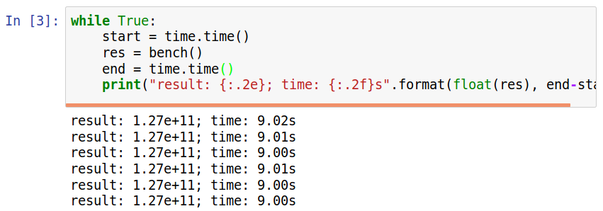
enddoA first Benchmark
Desktop PC (4 cores)


A first Benchmark
Cluster node (24 cores)

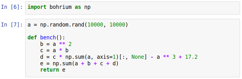
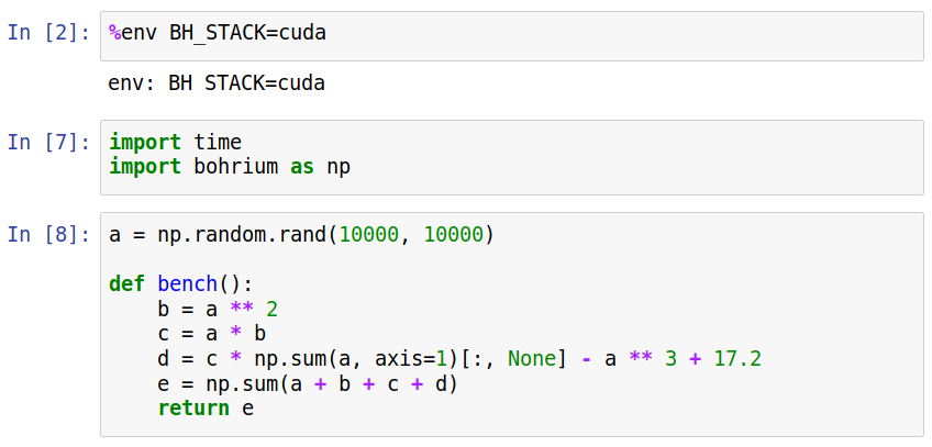
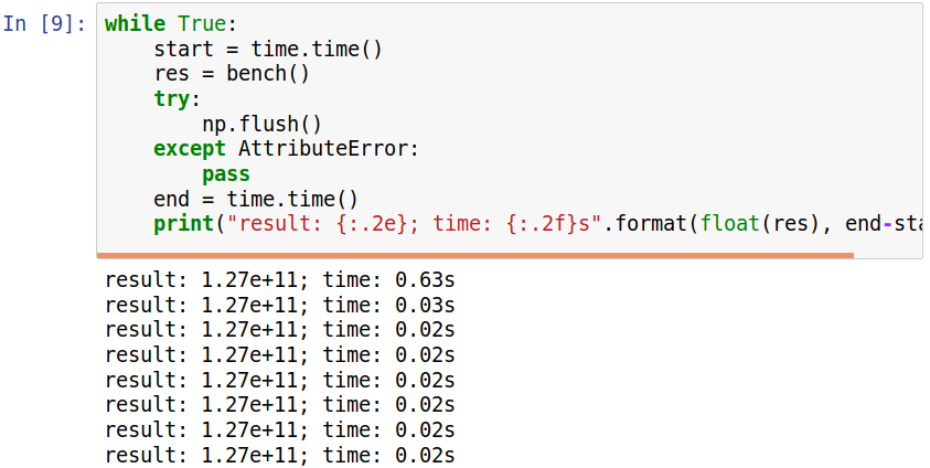
Bohrium
import bohrium as np
a = np.ones((100, 100))
a.sum()Provides a JIT compiler for NumPy code
Example:
#include <stdint.h>
#include <stdlib.h>
#include <stdbool.h>
#include <complex.h>
#include <tgmath.h>
#include <math.h>
void execute(double* __restrict__ a0, uint64_t vo0, uint64_t vs0_0, uint64_t vs0_1,
uint64_t vo1, uint64_t vs1_0, const double c1){
double t2;
t2 = 0;
#pragma omp parallel for reduction(+:t2)
for(uint64_t i0 = 0; i0 < 100; ++i0) {
double t1;
t1 = 0;
#pragma omp simd reduction(+:t1)
for(uint64_t i1 = 0; i1 < 100; ++i1) {
const uint64_t idx0= (vo0 +i0*vs0_0 +i1*vs0_1);
a0[idx0] = c1;
t1 += a0[idx0];
}
t2 += t1;
}
}
void launcher(void* data_list[], uint64_t offset_strides[], union dtype constants[]) {
double *a0 = data_list[0];
execute(a0, offset_strides[0], offset_strides[1], offset_strides[2],
offset_strides[3], offset_strides[4], constants[0].BH_FLOAT64);
}
OpenMP (CPU)
#pragma OPENCL EXTENSION cl_khr_fp64 : enable
#include <kernel_dependencies/complex_opencl.h>
#include <kernel_dependencies/integer_operations.h>
__kernel void execute(__global double* __restrict__ a0, __global double* __restrict__ a1,
ulong vo0, ulong vs0_0, ulong vs0_1, ulong vo1, ulong vs1_0,
const double c1) {
// The IDs of the threaded blocks:
const uint g0 = get_global_id(0); if (g0 >= 100) { return; } // Prevent overflow
{const ulong i0 = g0;
double s1;
s1 = 0;
for (ulong i1 = 0; i1 < 100; ++i1) {
const ulong idx0= (vo0 +i0*vs0_0 +i1*vs0_1);
a0[idx0] = c1;
s1 += a0[idx0];
}
a1[vo1 +i0*vs1_0] = s1;
}
}OpenCL (GPU)
Bohrium
Provides a JIT compiler for NumPy code
Bohrium
Provides a JIT compiler for NumPy code
Bohrium
Provides a JIT compiler for NumPy code
Bohrium
Provides a JIT compiler for NumPy code
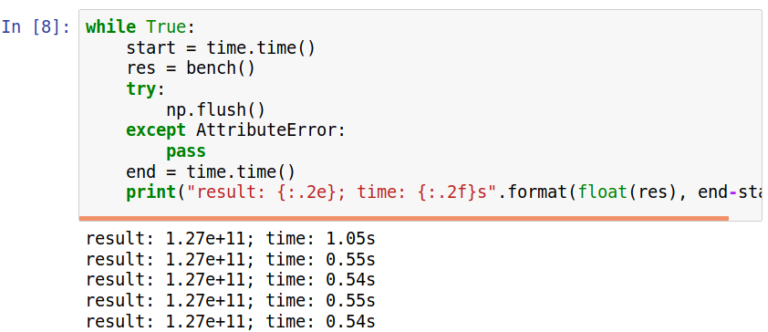
Looks better!
Desktop PC (4 cores)


Looks better!
Cluster Node (24 cores + NVIDIA Tesla P100)

So,
what can you do with it?
You can use it for Education

Southern Channel
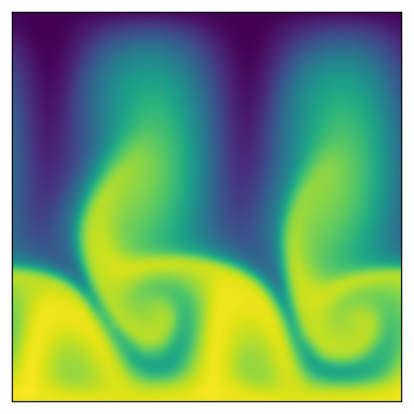
Eady Model
You can use it for Prototyping
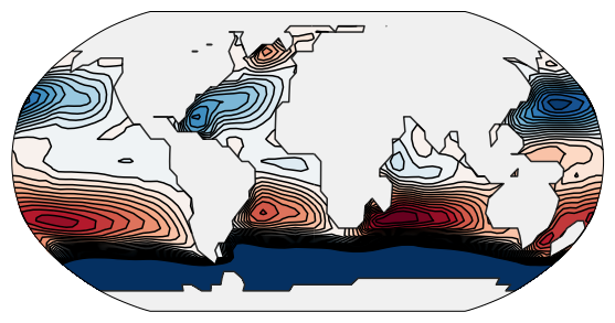
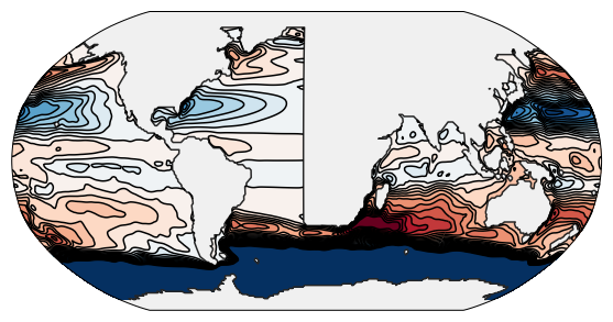
Global 4°x4° Model
You can use it for Research
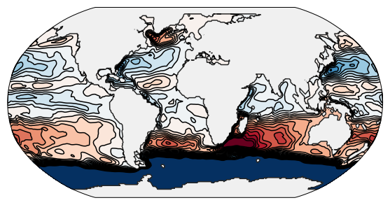
Global 1°x1° Model
Wave Propagation study
You can use it for Research
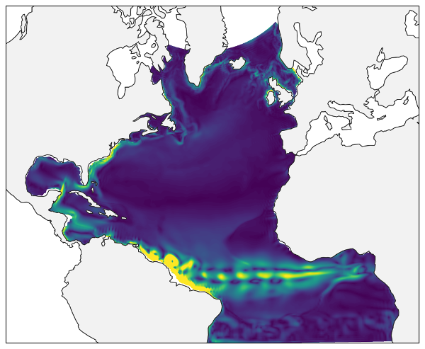
Regional Models
Open Issues
- More abstraction
vs.flux_east[1:-2, 2:-2,:] = \
	0.25 * (vs.u[1:-2, 2:-2, :, vs.tau] + vs.u[2:-1, 2:-2, :, vs.tau]) \
* (vs.utr[1:-2, 2:-2, :] + vs.utr[1:-2, 2:-2, :])vs.flux_east.update(
on('t', vs.u[..., vs.tau]) * on('t', vs.utr)
)Draft
- xarray integration
- Explore other (distributed) backends: Dask, Theano, CuPy?
- Veras, the versatile atmosphere simulator?

veros.readthedocs.org
References
Summary
- Core routines based on pyOM2
- Fast-ish on CPU and GPU through Bohrium (single node only)
- Pythonic, object-oriented frontend
- Runs idealized and realistic models
- Most of all: versatile!
- Eden, Carsten (2016). “Closing the energy cycle in an ocean model”. In: Ocean Modelling 101
- Kristensen, Mads RB, et al. (2013). “Bohrium: un-modified NumPy code on CPU, GPU, and cluster”. In: Python for High Performance and Scientific
Computing (PyHPC 2013). - Larsen, Mads Ohm et al. (2016). “Current Status and Directions for the Bohrium Runtime System”. In:
Compilers for Parallel Computing 2016.
Bonus slides
Other Python Niceties
- No explicit parallelization
- AMG streamfunction solvers
- Modular diagnostics
- Compressed, threaded I/O
- Dynamic backend handling
- Object-oriented, Pythonic configuration
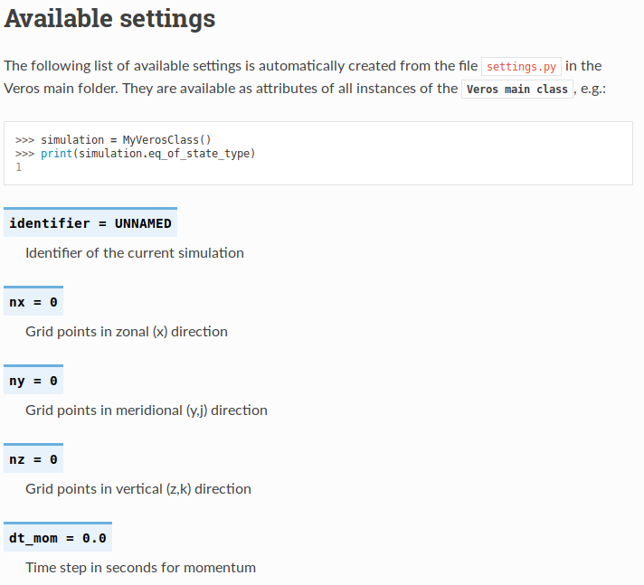
- Self-documentation
- Automated tests
General
Backend
Poisson solver benchmark

Desktop PC
Cluster Node
with pyAMG
Example configuration
from veros import Veros, veros_method


class ACC(Veros):
    """A model using spherical coordinates with a partially closed domain representing the Atlantic and ACC.

    Wind forcing over the channel part and buoyancy relaxation drive a large-scale meridional overturning circulation.

    This setup demonstrates:
     - setting up an idealized geometry
     - updating surface forcings
     - basic usage of diagnostics

    `Adapted from pyOM2 <https://wiki.cen.uni-hamburg.de/ifm/TO/pyOM2/ACC%202>`_.
    """
    @veros_method
    def set_parameter(self):
        self.identifier = "acc"

        self.nx, self.ny, self.nz = 30, 42, 15
        self.dt_mom = 4800
        self.dt_tracer = 86400 / 2.
        self.runlen = 86400 * 365

        self.coord_degree = True
        self.enable_cyclic_x = True

        self.congr_epsilon = 1e-12
        self.congr_max_iterations = 5000

        self.enable_neutral_diffusion = True
        self.K_iso_0 = 1000.0
        self.K_iso_steep = 500.0
        self.iso_dslope = 0.005
        self.iso_slopec = 0.01
        self.enable_skew_diffusion = True


        self.enable_hor_friction = True
        self.A_h = (2 * self.degtom)**3 * 2e-11
        self.enable_hor_friction_cos_scaling = True
        self.hor_friction_cosPower = 1

        self.enable_bottom_friction = True
        self.r_bot = 1e-5

        self.enable_implicit_vert_friction = True

        self.enable_tke = True
        self.c_k = 0.1
        self.c_eps = 0.7
        self.alpha_tke = 30.0
        self.mxl_min = 1e-8
        self.tke_mxl_choice = 2
        # self.enable_tke_superbee_advection = True

        self.K_gm_0 = 1000.0
        self.enable_eke = True
        self.eke_k_max = 1e4
        self.eke_c_k = 0.4
        self.eke_c_eps = 0.5
        self.eke_cross = 2.
        self.eke_crhin = 1.0
        self.eke_lmin = 100.0
        self.enable_eke_superbee_advection = True
        self.enable_eke_isopycnal_diffusion = True

        self.enable_idemix = True
        self.enable_idemix_hor_diffusion = True
        self.enable_eke_diss_surfbot = True
        self.eke_diss_surfbot_frac = 0.2
        self.enable_idemix_superbee_advection = True

        self.eq_of_state_type = 3

    @veros_method
    def set_grid(self):
        ddz = np.array([50., 70., 100., 140., 190., 240., 290., 340.,
                        390., 440., 490., 540., 590., 640., 690.])
        self.dxt[...] = 2.0
        self.dyt[...] = 2.0
        self.x_origin = 0.0
        self.y_origin = -40.0
        self.dzt[...] = ddz[::-1] / 2.5

    @veros_method
    def set_coriolis(self):
        self.coriolis_t[:, :] = 2 * self.omega * np.sin(self.yt[None, :] / 180. * self.pi)

    @veros_method
    def set_topography(self):
        x, y = np.meshgrid(self.xt, self.yt, indexing="ij")
        self.kbot[...] = np.logical_or(x > 1.0, y < -20).astype(np.int)

    @veros_method
    def set_initial_conditions(self):
        # initial conditions
        self.temp[:, :, :, 0:2] = ((1 - self.zt[None, None, :] / self.zw[0]) * 15 * self.maskT)[..., None]
        self.salt[:, :, :, 0:2] = 35.0 * self.maskT[..., None]

        # wind stress forcing
        taux = np.zeros(self.ny + 4, dtype=self.default_float_type)
        taux[self.yt < -20] = 1e-4 * np.sin(self.pi * (self.yu[self.yt < -20] - self.yu.min()) / (-20.0 - self.yt.min()))
        taux[self.yt > 10] = 1e-4 * (1 - np.cos(2 * self.pi * (self.yu[self.yt > 10] - 10.0) / (self.yu.max() - 10.0)))
        self.surface_taux[:, :] = taux * self.maskU[:, :, -1]

        # surface heatflux forcing
        self._t_star = 15 * np.ones(self.ny + 4, dtype=self.default_float_type)
        self._t_star[self.yt < -20] = 15 * (self.yt[self.yt < -20] - self.yt.min()) / (-20 - self.yt.min())
        self._t_star[self.yt > 20] = 15 * (1 - (self.yt[self.yt > 20] - 20) / (self.yt.max() - 20))
        self._t_rest = self.dzt[None, -1] / (30. * 86400.) * self.maskT[:, :, -1]

        if self.enable_tke:
            self.forc_tke_surface[2:-2, 2:-2] = np.sqrt((0.5 * (self.surface_taux[2:-2, 2:-2] + self.surface_taux[1:-3, 2:-2]))**2
                                                      + (0.5 * (self.surface_tauy[2:-2, 2:-2] + self.surface_tauy[2:-2, 1:-3]))**2)**(1.5)

        if self.enable_idemix:
            self.forc_iw_bottom[...] = 1e-6 * self.maskW[:, :, -1]
            self.forc_iw_surface[...] = 1e-7 * self.maskW[:, :, -1]

    @veros_method
    def set_forcing(self):
        self.forc_temp_surface[...] = self._t_rest * (self._t_star - self.temp[:, :, -1, self.tau])

    @veros_method
    def set_diagnostics(self):
        self.diagnostics["snapshot"].output_frequency = 86400 * 10
        self.diagnostics["averages"].output_variables = (
            "salt", "temp", "u", "v", "w", "psi", "surface_taux", "surface_tauy"
        )
        self.diagnostics["averages"].output_frequency = 365 * 86400.
        self.diagnostics["averages"].sampling_frequency = self.dt_tracer * 10
        self.diagnostics["overturning"].output_frequency = 365 * 86400. / 48.
        self.diagnostics["overturning"].sampling_frequency = self.dt_tracer * 10
        self.diagnostics["tracer_monitor"].output_frequency = 365 * 86400. / 12.
        self.diagnostics["energy"].output_frequency = 365 * 86400. / 48
        self.diagnostics["energy"].sampling_frequency = self.dt_tracer * 10


if __name__ == "__main__":
    simulation = ACC()
    simulation.setup()
    simulation.run()
Veros@AMS
By Dion Häfner
Veros@AMS
I presented Veros at the 89th annual meeting of the American Meteorological Society (AMS).
