Data Wrangling II

Outline
Review
Grouped operations
Joining data.frames
{review}
Steps for analysis
Articulate question of interest
Translate your question into code
Execute your program
{dplyr}
DPLYR's Data Manipulation Grammar
Select the columns of interest
Filter down to rows of interest
Mutate new columns
# Arguments are data.frame, then comma separated column names
my_cols <- select(df, col1, col2, col3)
# Arguments are data.frame, then comma separated boolean operators
my_rows <- filter(df, col1 > col2, col2 < col3, col4 == "hello")# Arguments are data.frame, then comma separated sorting columns
sorted_df <- arrange(df, col1, desc(col2))Arrange your data by a column's values
# Arguments are data.frame, then comma separated new columns
new_df <- mutate(df, combined = col1 + col2, diff = col1 - col2)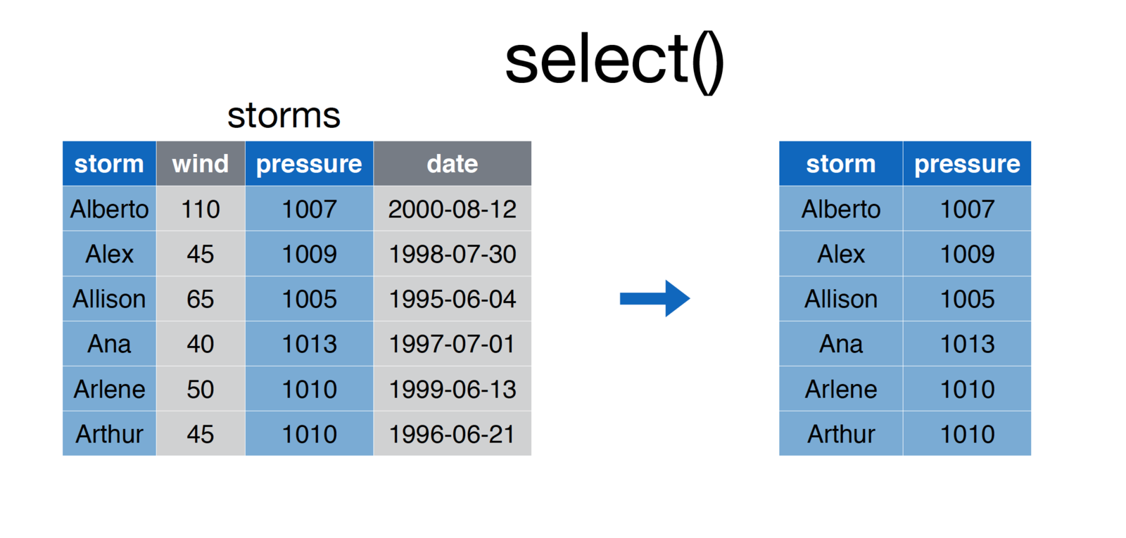
credit: Nathan Stephens, Rstudio
# Select storm and pressure columns from storms dataframe
storms <- select(storms, storm, pressure)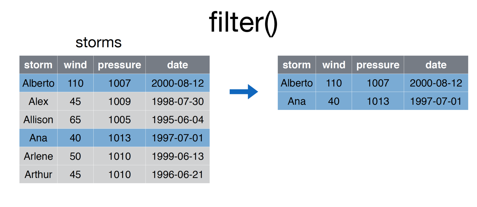
credit: Nathan Stephens, Rstudio
# Filter down storms to storms with name Ana or Alberto
storms <- filter(storms, storm %in% c('Ana', 'Alberto')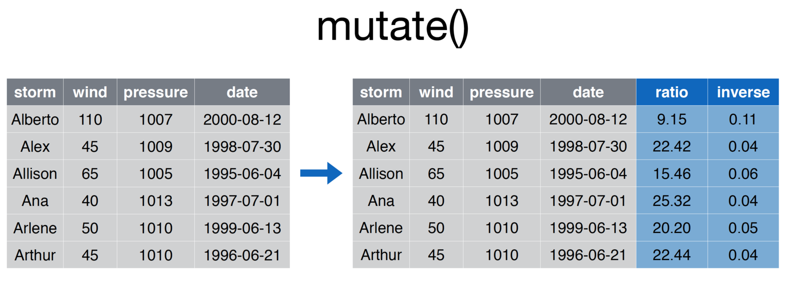
credit: Nathan Stephens, Rstudio
# Add ratio and inverse ratio columns
storms <- mutate(storms, ratio = pressure/wind, inverse = 1/ratio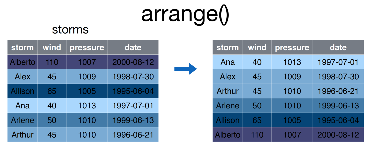
credit: Nathan Stephens, Rstudio
# Arrange storms by wind
storms <- arrange(storms, wind)
credit: Nathan Stephens, Rstudio
Additional funcitonality
Select helper functions
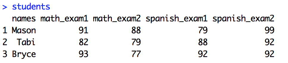
# Make a data.frame
students <- data.frame(
  names=c('Mason', 'Tabi', 'Bryce'),
  math_exam1 = c(91, 82, 93),
  math_exam2 = c(88, 79, 77),
  spanish_exam1 = c(79, 88, 92),
  spanish_exam2 = c(99, 92, 92)
)

# Select students + math grades
math_grades <- select(students, names, math_exam1, math_exam2)

# Better yet!
math_grades <- select(students, names, contains("math"))

# See also: starts_with, ends_with, matches
Additional funcitonality
Using select_ (or filter_, mutate_, etc.)
# Make a data.frame
students <- data.frame(
  names=c('Mason', 'Tabi', 'Bryce'),
  math_exam1 = c(91, 82, 93),
  math_exam2 = c(88, 79, 77),
  spanish_exam1 = c(79, 88, 92),
  spanish_exam2 = c(99, 92, 92)
)

# Why is this useful?
exam_of_interest <- 'math_exam1'
exam_grades <- select_(students, 'names', exam_of_interest)
{exercise 1}
today's exercises inspired by Intro to dplyr documentation
Summarise
Great for calculating summaries
# Compute values of interest
summarise(students,
            mean_math1 = mean(math_exam1),
            mean_math2 = mean(math_exam2),
            mean_math_scores=mean((math_exam1 + math_exam2) / 2)
          )
Calculate one value from a set of values
# Compute values of interest
summarise(students,
            num_students = n()
          )
A nifty trick
Grouped operations
Group data by column values
Ask questions that compare computed values
Data needs to be in the right format
Data shapes
Wide data
Long data
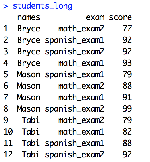
Long data will let you group by column and compare computed values
Reshaping
# Reshape students from wide to long format (just FYI)
varying <- c('math_exam1', 'spanish_exam1', 'math_exam2', 'spanish_exam2')
students_long <- reshape(students,
        timevar='exam',
        idvar='names',
        v.names = 'score',
        times=varying,
        varying=varying,
        direction="long") %>% arrange(names, score)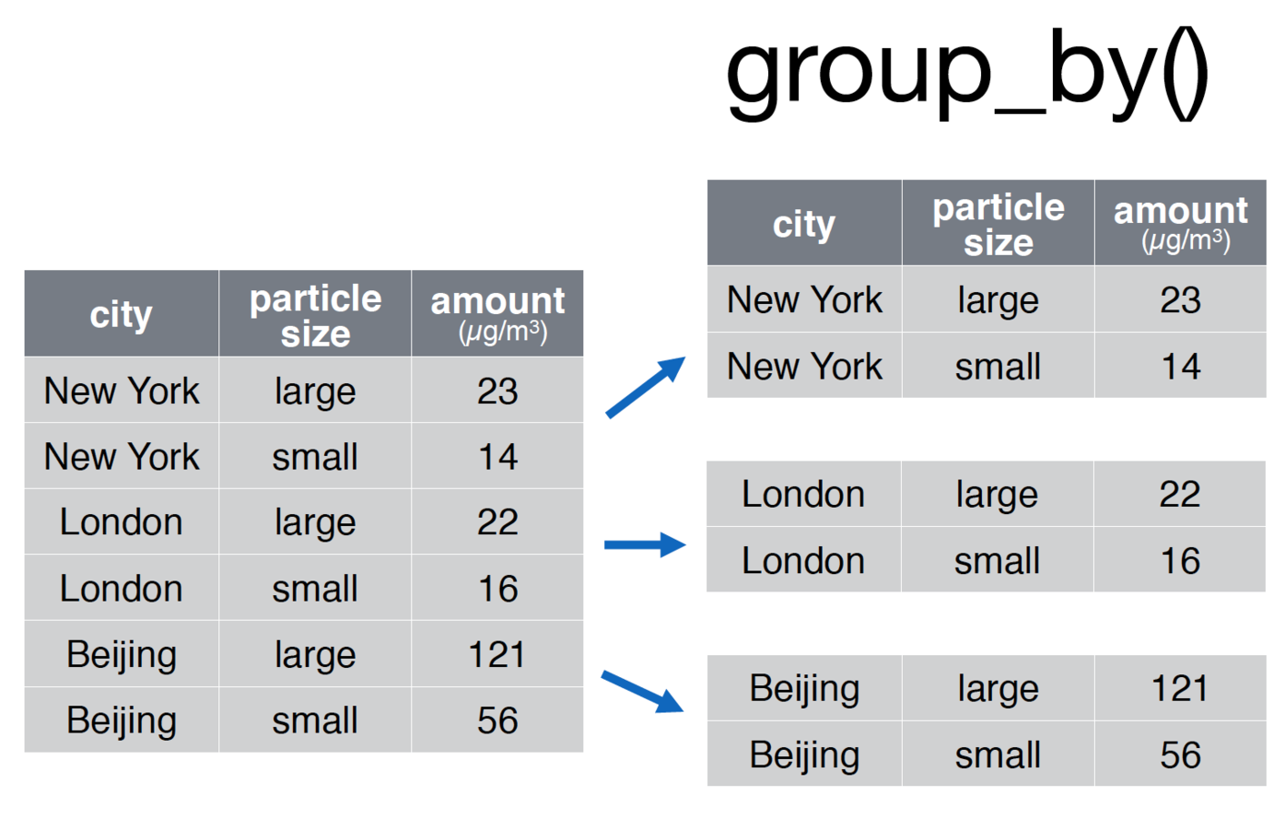
credit: Nathan Stephens, Rstudio
# Group the pollution data.frame by city for comparison
pollution <- group_by(pollution, city)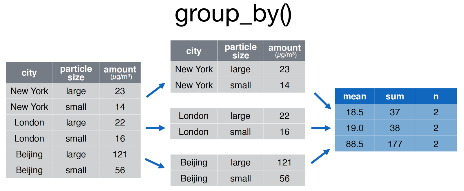
credit: Nathan Stephens, Rstudio
# Group the pollution data.frame by city for comparison
pollution <- group_by(pollution, city) %>%
               summarise(
                mean = mean(amount, na.rm = TRUE),
                sum = sum(amount, na.rm = TRUE),
                n = n()
            )
Grouped data
Which student has the highest average?
Which exam was most difficult?
Which student has the highest math average?
Which Spanish exam had the lowest average score?
{exercise 2}
Joins
Joins
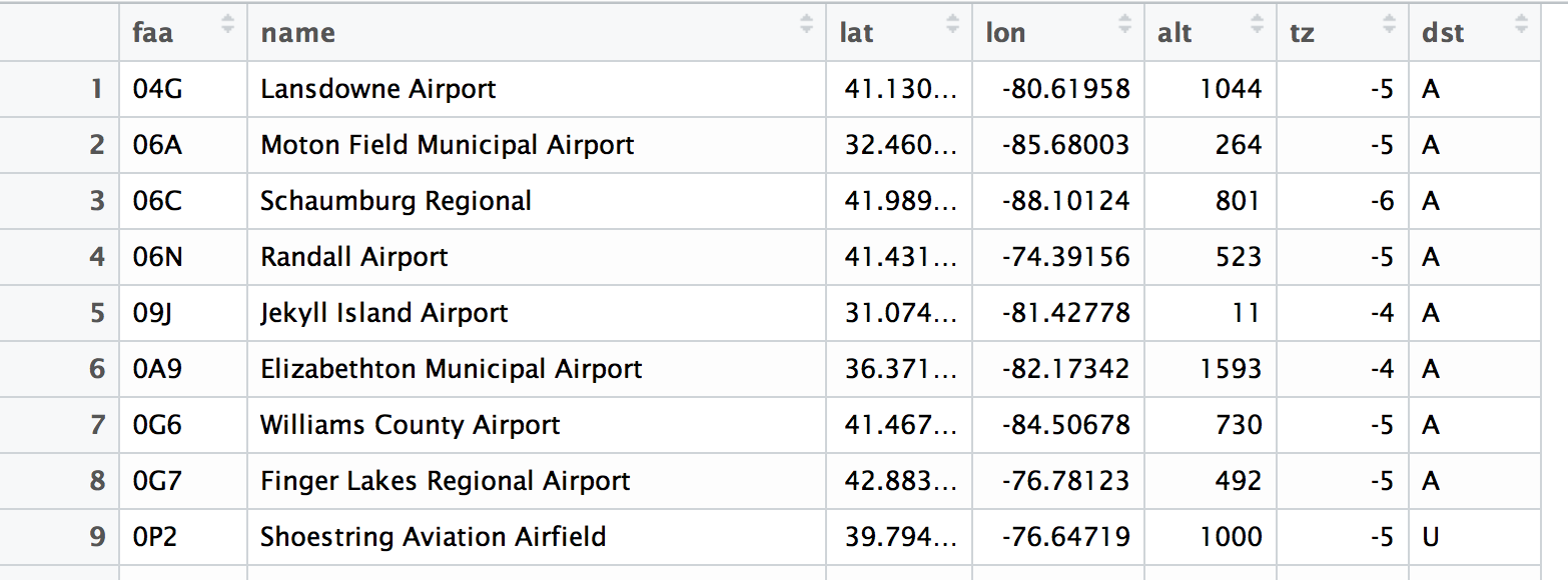
Why is this airport information stored in a separate table?
Joins
Allow you to combine columns from multiple data sources
Foundation of relational databases
Specify the identifying columns shared by the columns
Many types of joins (easy to confuse)
Left-joins
Join two data.frames by shared identifier(s)
# These could be different!
joined_x_y <- left_join(x, y, by='identifier')
joined_y_x <- left_join(x, y, by='identifier')
Order matters!
Returns all rows in x, and all columns for x and y
# Join x and y by 'identifier'
joined <- left_join(x, y, by='identifier')
Left-joins
# Student majors
majors <- data.frame(
  student_id=c(1, 2, 3),
  major=c('sociology', 'math', 'biology')
)

# Student contact info
contact_info <- data.frame(
  student_id=c(1,2),
  cell=c('382-842-5873', '593-254-5834')
)

# Left join
joined <- left_join(majors, contact_info, by='student_id')

# Order matters!
joined <- left_join(contact_info, majors, by='student_id')
{exercise 3}
Assignments
Assignment-4: Data wrangling (due Wed. 2/3)
data-wrangling-2
By Michael Freeman


