
russtedrake PRO
Roboticist at MIT and TRI
Follow live at https://slides.com/d/giJbYyg/live
(or later at https://slides.com/russtedrake/fall23-lec04)
MIT 6.4210/2: Robotic Manipulation
Fall 2023, Lecture 4
Kinematic Jacobian: \( {}^WV^G = J^{G}(q) v \)
\( v = [J^{G}(q)]^{-1} {}^WV^G \)
spatial velocity
generalized velocity
Example: Gimbal Lock
plant = MultibodyPlant(time_step = 0.0)
Parser(plant).AddModelFromFile(FindResourceOrThrow(
	"drake/examples/manipulation_station/models/061_foam_brick.sdf"))
plant.Finalize()
brick = plant.GetBodyByName("base_link")

context = plant.CreateDefaultContext()
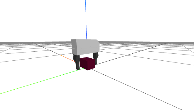
What is \(X^B\) ?
X_B = plant.EvalBodyPoseInWorld(brick, context)What is \(q\) ?
q = plant.GetPositions(context)Kinematic "Jacobian"
angular velocity
translational velocity
Q: How do we represent angular velocity, \(\omega^B\)??
A: Unlike 3D rotations, here 3 numbers are sufficient and efficient; so we use the same representation everywhere.
note the typesetting
plant = MultibodyPlant(time_step = 0.0)
Parser(plant).AddModelFromFile(FindResourceOrThrow(
	"drake/examples/manipulation_station/models/061_foam_brick.sdf"))
plant.Finalize()
brick = plant.GetBodyByName("base_link")

context = plant.CreateDefaultContext()
What size is \(v\) ?
v = plant.GetVelocities(context)What size is \(q\) ?
q = plant.GetPositions(context)v = plant.MapQDotToVelocity(context, qdot)qdot = plant.MapVelocityToQDot(context, v)For any MultibodyPlant (not just a single body):
\( v = [J^{G}(q)]^{-1} {}^WV^G \)
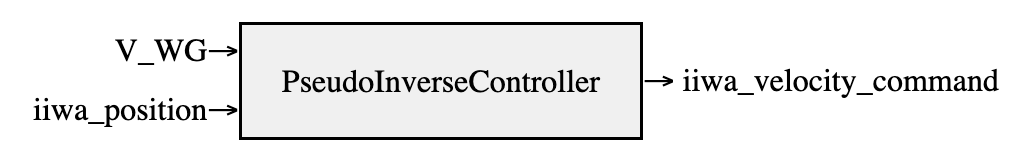
class PseudoInverseController(LeafSystem):
    def __init__(self, plant):
        LeafSystem.__init__(self)
        self.V_G_port = self.DeclareVectorInputPort("V_WG", 6)
        self.q_port = self.DeclareVectorInputPort("iiwa.position", 7)
        self.DeclareVectorOutputPort("iiwa.velocity", 7, self.CalcOutput)

    def CalcOutput(self, context, output):
        V_G = self.V_G_port.Eval(context)
        q = self.q_port.Eval(context)
        self._plant.SetPositions(self._plant_context, self._iiwa, q)
        J_G = self._plant.CalcJacobianSpatialVelocity(
            self._plant_context,
            JacobianWrtVariable.kV,
            self._G,
            [0, 0, 0],
            self._W,
            self._W,
        )
        J_G = J_G[:, self.iiwa_start : self.iiwa_end + 1]  # Only iiwa terms.
        v = np.linalg.pinv(J_G).dot(V_G)
        output.SetFromVector(v)
prog = MathematicalProgram()
x = prog.NewContinuousVariables(2)
prog.AddConstraint(x[0] + x[1] == 1)
prog.AddConstraint(x[0] <= x[1])
prog.AddCost(x[0] ** 2 + x[1] ** 2)
result = Solve(prog)By russtedrake
MIT Robotic Manipulation Fall 2023 http://manipulation.csail.mit.edu


