Discrete + continuous optimization

MIT 6.821: Underactuated Robotics

Spring 2023, Lecture 17

Follow live at https://slides.com/d/Yp1UjL4/live
(or later at https://slides.com/russtedrake/spring24-lec17)

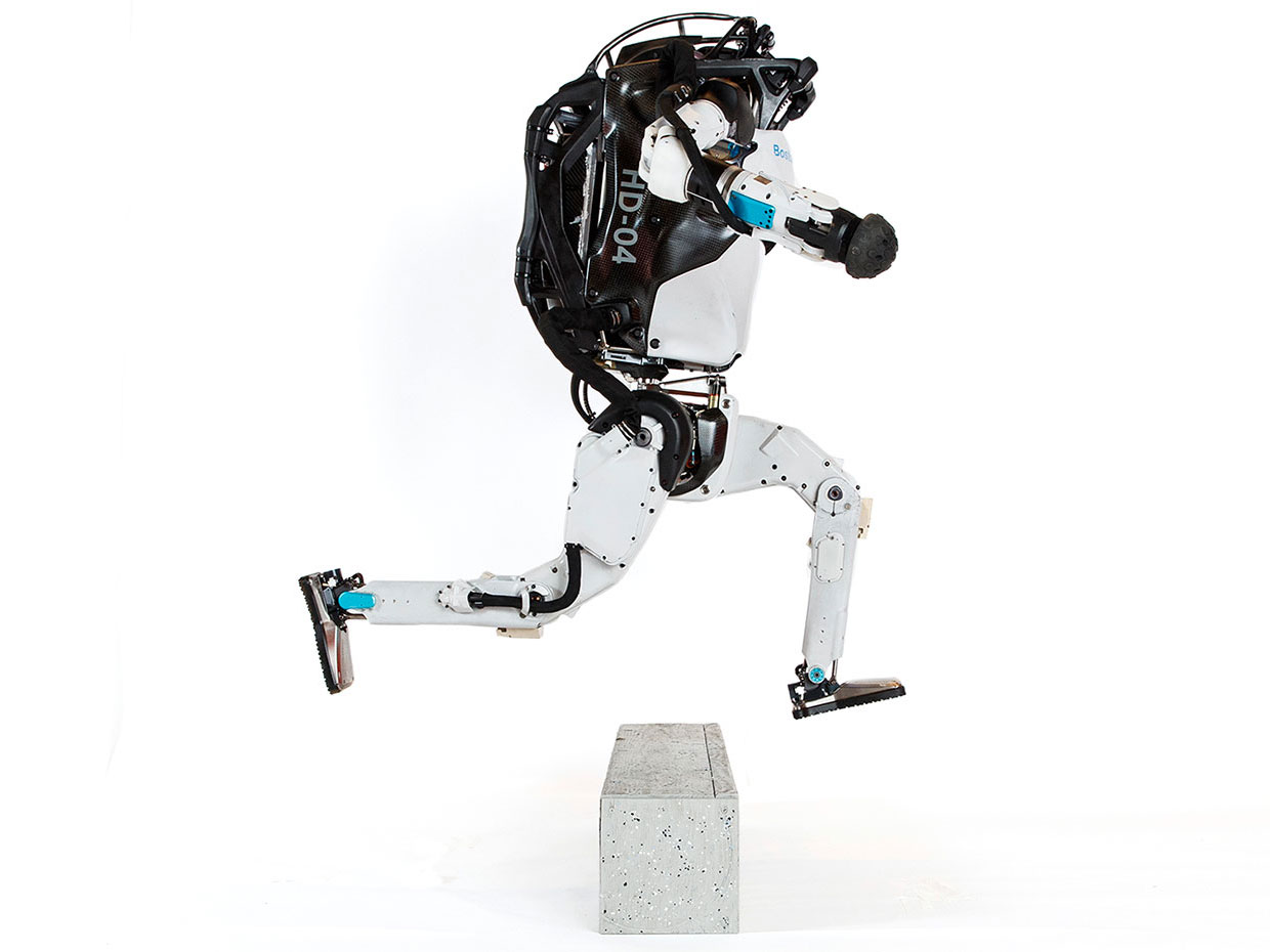
Image credit: Boston Dynamics
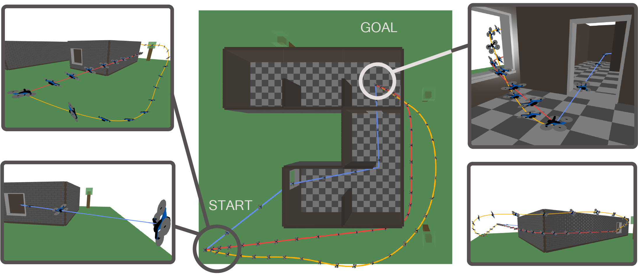
Running example: Shortest path around an obstacle

start

goal

  1. Combinatorial (e.g. over homotopy classes)
  2. Smooth optimization (over curves)

Two aspects of the motion planning problem:

start

goal

Motion planning as a (nonconvex) optimization

\begin{aligned} \min_{x_0, ..., x_N} \quad & \sum_{n=0}^{N-1} | x_{n+1} - x_n|_2^2 & \\ \text{subject to} \quad & x_0 = x_{start} \\ & x_N = x_{goal} \\ & |x_n|_1 \ge 1 & \forall n \end{aligned}

start

goal

fixed number of samples

collision-avoidance

(outside the \(L^1\) ball)

nonconvex

Planning as a mixed-integer convex program

\begin{aligned} \min_{x_0, ..., x_N} \quad & \sum_{n=0}^{N-1} | x_{n+1} - x_n|_2^2 & \\ \text{subject to} \quad & x_0 = x_{start} \\ & x_N = x_{goal} \end{aligned}
[1,1]^T x_n \ge 1 \quad \textbf{or} \quad [1,1]^T x_n \le -1 \quad \textbf{or} \\ [1,-1]^T x_n \ge 1 \quad \textbf{or} \quad [1,-1]^T x_n \le -1, \quad \forall n.

goal

start

[1,1]

disjunctive

constraints

[1,1]^T x_n \ge 1

Mixed-integer programs

\begin{aligned} \underset{x, b}{\text{minimize}} \quad & f(x, b) \\ \text{subject to} \quad & g(x, b) \le 0 \\ & b_i \in \{0, 1\}, \forall i \end{aligned}
0 \le b_i \le 1

"Convex relaxation" replaces this with:

"Mixed-integer convex" iff \(f\) and \(g\) are convex.

Convex relaxation is "tight" when the relaxed solution is a solution to the original problem.

Branch and bound

b_0 = 0.9, b_1 = 0.4
b_0 = 1
b_0 = 0
b_1 = 1
b_1 = 0

Convex relaxations provide lower bounds

Feasible solutions provide upper bounds

convex

convex

convex

convex

convex

\begin{aligned} \underset{x, b}{\text{minimize}} \quad & f(x, b) \\ \text{subject to} \quad & g(x, b) \le 0 \\ & b_i \in \{0, 1\}, \forall i \end{aligned}

Branch and bound performance

  • Number of integer variables
  • "Tightness" of the convex relaxation 
  • Motion planning transcription:

\(\Rightarrow\) Long solve times.

b_0 = 0.9, b_1 = 0.4
b_0 = 1
b_0 = 0
b_1 = 1
b_1 = 0
  • Too many integer variables (false combinatorial complexity)
  • Disjunctive programming leads to "loose" relaxations

Traditional Shortest Path as a Linear Program (LP)

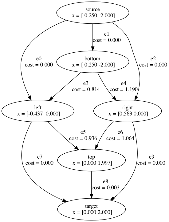
\(\varphi_{ij} = 1\) if the edge \((i,j)\) in shortest path, otherwise \(\varphi_{ij} = 0.\)

\(c_{ij} \) is the (constant) length of edge \((i,j).\)

\begin{aligned} \min_{\varphi} \quad & \sum_{(i,j) \in E} c_{ij} \varphi_{ij} \\ \mathrm{s.t.} \quad & \sum_{j \in E_i^{out}} \varphi_{ij} + \delta_{ti} = \sum_{j \in E_i^{in}} \varphi_{ji} + \delta_{si}, && \forall i \in V, \\ & \varphi_{ij} \in \{0, 1\}, && \forall (i,j) \in E. \end{aligned}

"flow constraints"

binary relaxation

path length

\begin{aligned} \min_{\varphi} \quad & \sum_{(i,j) \in E} c_{ij} \varphi_{ij} \\ \mathrm{s.t.} \quad & \sum_{j \in E_i^{out}} \varphi_{ij} + \delta_{ti} = \sum_{j \in E_i^{in}} \varphi_{ji} + \delta_{si}, && \forall i \in V, \\ & \varphi_{ij} \ge 0, && \forall (i,j) \in E. \end{aligned}

Graphs of Convex Sets


  • For each \(i \in V:\)
    • Compact convex set \(X_i \subset \R^d\)
    • A point \(x_i \in X_i \) 
  • Edge length given by a convex function \[ \ell(x_i, x_j) \]

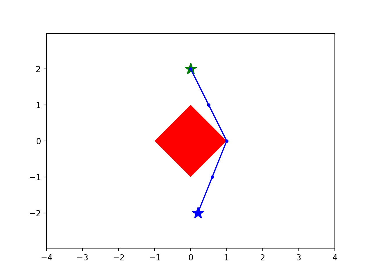
Note: The blue regions are not obstacles.

New shortest path formulation

\begin{aligned} \min_{\varphi} \quad & \sum_{(i,j) \in E} c_{ij} \varphi_{ij} \\ \mathrm{s.t.} \quad & \sum_{j \in E_i^{out}} \varphi_{ij} + \delta_{ti} = \sum_{j \in E_i^{in}} \varphi_{ji} + \delta_{si}, && \forall i \in V, \\ & \varphi_{ij} \geq 0, && \forall (i,j) \in E. \end{aligned}

Classic shortest path LP

\begin{aligned} \min_{\varphi,x} \quad & \sum_{(i,j) \in E} \ell_{ij}(x_i, x_j) \varphi_{ij} \\ \mathrm{s.t.} \quad & x_i \in X_i, && \forall i \in V, \\ & \sum_{j \in E_i^{out}} \varphi_{ij} + \delta_{ti} = \sum_{j \in E_i^{in}} \varphi_{ji} + \delta_{si} \le 1, && \forall i \in V, \\ & \varphi_{ij} \geq 0, && \forall (i,j) \in E. \end{aligned}

now w/ Convex Sets

New shortest path formulation

\begin{aligned} \min_{\varphi,x} \quad & \sum_{(i,j) \in E} \ell_{ij}(x_i, x_j) \varphi_{ij} \\ \mathrm{s.t.} \quad & x_i \in X_i, && \forall i \in V, \\ & \sum_{j \in E_i^{out}} \varphi_{ij} + \delta_{ti} = \sum_{j \in E_i^{in}} \varphi_{ji} + \delta_{si} \le 1, && \forall i \in V, \\ & \varphi_{ij} \geq 0, && \forall (i,j) \in E. \end{aligned}

Non-negative scaling of a convex set is still convex (e.g. via "perspective functions")

Achieved orders of magnitude speedups.

Randomized rounding

b_0 = 0.98, b_1 = 0.02, b_2 = 0.97, b_3 = 0.004, ...

convex

Motion planning with Graph of Convex Sets (GCS)

\ell_{i,j}(x_i, x_j) = |x_i - x_j|_2

start

goal

Motion planning with Graph of Convex Sets (GCS)

This is the convex relaxation

(it is tight!).

          is the convex relaxation.  (it's tight!)

Previous formulations were intractable; would have required \( 6.25 \times 10^6\) binaries.

  • When sets \( X_i \) are points, reduces to standard LP formulation of the shortest path (known to be tight).


  • There are instances of this problem that are NP-hard.
  • We give simple examples where relaxation is not tight.

  • Can add (piecewise-affine) dynamic constraints on pairs \( (x_i,x_j). \)

Remarks

Ex: Minimum-time double integrator

Example: "Footstep planning" with \(x_{n+1}=Ax_n + Bu_n\)

Previous best formulations New formulation
Lower Bound
(from convex relaxation)
7% of MICP 80% of MICP

Dynamic planning through contact

Planning through contact for Planar Pushing

Planning through contact for general manipulation

Lecture 17: Discrete (combinatorial) + continuous optimization

By russtedrake

Lecture 17: Discrete (combinatorial) + continuous optimization

MIT Underactuated Robotics Spring 2024 http://underactuated.csail.mit.edu

  • 103