An introduction to gradient descent algorithms

Abdellah CHKIFA
abdellah.chkifa@um6p.ma

Outline
1. Gradient Descent
- Gradient Descent
- Linear regression
- Batch Gradient Descent
- Stochastic Gradient Descent
2. Back-propagation
- Logistic regression
- Soft-max regression
- Neural networks
- Deep neural networks
Gradient Descent: an intuitive algorithm

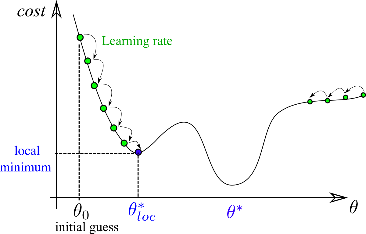
objective function (also called loss function or cost function etc.)
initial guess
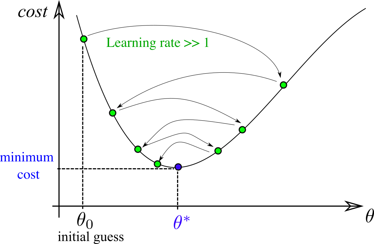
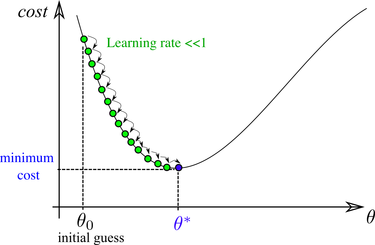
Importance of learning rate


We consider GD applied to
with
and rates
Gradient Descent: a convergence theorem
initial guess
f convex:
f L-smooth:
Suppose that f is convex and L-smooth. The gradient descent algorithm with η < 1/L converge to θ* and yields the convergence rate
Theorem
Gradient Descent: a convergence theorems
initial guess
f μ-strongly convex:
suppose that f is μ-strongly convex and L-smooth. The gradient descent algorithm with η < 1/L converge to θ* with
Theorem
μ-strong convexity can be weakened to Polyak-Lojasiewicz Condition 🔗
- Easy to implement.
- Each iteration is (relatively!) cheap, computation of one gradient.
- Can be very fast for smooth objective functions, as shown.
- The coefficient L may not be accurately estimated.
- => Choice of small learning rate.
- Concrete objective functions are usually not strongly convex nor convex.
- GD does not handle non-differentiable functions (biggest downside).
Pros and Cons
Reference
https://www.stat.cmu.edu/~ryantibs/convexopt/