Cotraining for Diffusion Policies
Aug 15, 2024
Adam Wei
Agenda
- Brief overview of Diffusion Policy
- Defining cotraining
- Problem statement
- Main experiments and results
- Discussion and ablations
Behavior Cloning

Behavior cloning (Diffusion Policy) can solve many robot tasks
...when data is available
Diffusion Policy Overview
Goal:
- Given data from an expert policy, p(A | O)...
- Learn a generative model to sample from p(A | O).
Diffusion Policy:
- Learn a denoiser / score function for p(A | O) and sample with diffusion
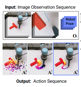
Diffusion Policy Overview
Training loss:
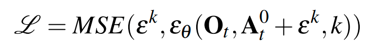
Condition on observations O by passing it as an input to the denoiser.
Sampling Procedure
Train with DDPM, sample with DDIM (faster inference)
Cotraining
Robot Poses

O
A


Robot Poses
A
O
Ex: From a human demonstrator
Ex: From GCS
Cotraining
- High quality data from the target distribution
- Expensive to collect
- Not the target distribution, but still informative data
- Scalable to collect
Cotraining: Use both datasets to train a model that maximizes some test objective
- Model: Diffusion Policy
- Test objective: Empirical success rate on a planar pushing task
Vanilla Cotraining: Mixtures
Cotraining: Use both datasets to train a Diffusion Policy that maximizes empirical success rate
Dataset Mixture: to sample from :
- Sample from with probability
- Sample from with probability
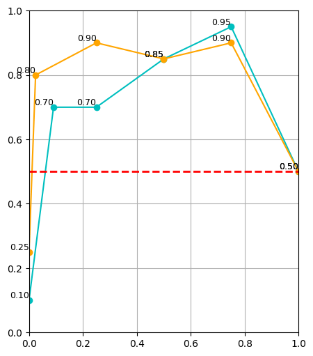
Preliminary Results: 50 real demos
SR= 10/20
SR= 19/20
SR= 14/20
Mixing ratio is important for good performance!
Preliminary Results: 10 real demos
SR= 2/20
SR= 3/20
SR= 14/20
The data scale affects the optimal mixing ratio!
Problem Statement
1. How do different data scales and mixing ratios affect policy performance (success rate)?
2. How do different distribution shifts in the simulated data affect the optimal mixing ratio and policy performance?
- i.e. What properties should we care about in our sim data?
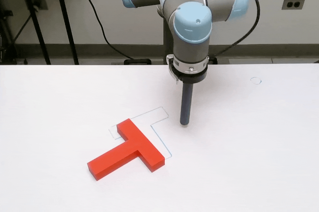
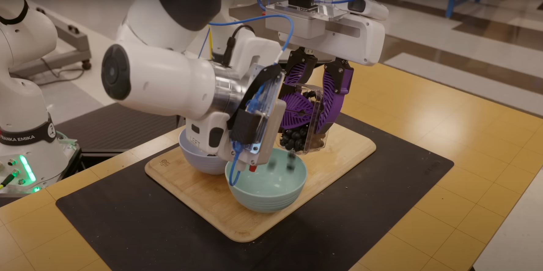
Experiments: T-Pushing
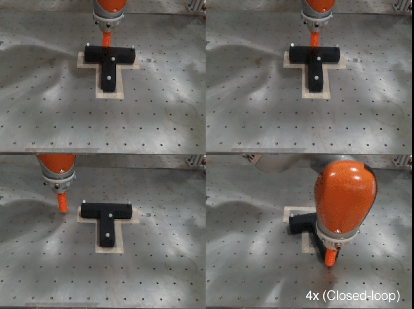
Task: Push a T-object from any initial planar pose within the robot's workspace to a pre-specified target pose.
Planar pushing is the simplest task that captures the broader challenges in manipulation.
- Planning and decision-making
- Contact dynamics
- Control from RGB
- Extenable to multi-task, language guidance, etc
Experiments: Data Collection
Real world data: teleoperation
Sim data:
- Generate plans with Bernhard's algorithm
- Clean data
- Replay and render the plans in Drake
Experiments: Data Collection

Experiments: Part 1
1. How do different data scales and mixing ratios affect the success rate of co-trained policies?
Experiments: Training and Eval
- Train for ~2 days on a single Supercloud V100
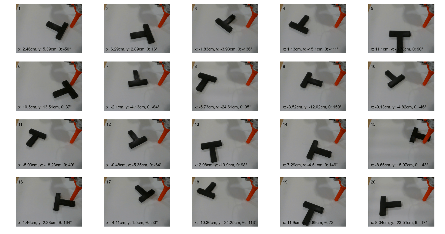
- Evaluate performance on 20 trials from matched initial conditions
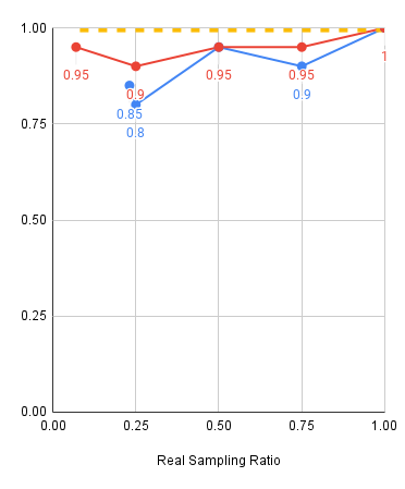
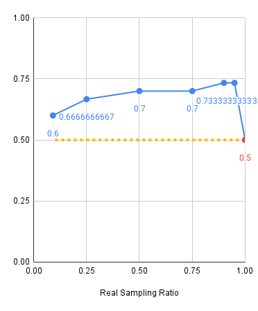
Experiments: Results
Red: 2000 sim demos, Blue: 500 sim demos, Yellow: Real only baseline
Experiments: Results
Experiments: Key Takeaways
Mixing ratio takeaways:
- Policy performance is sensitive to alpha, especially in low data regime
- Smaller real dataset => smaller alpha
- Larger real dataset => larger alpha
- If there is sufficient real data, sim data will not help. It also isn't detrimental:
Experiments: Results
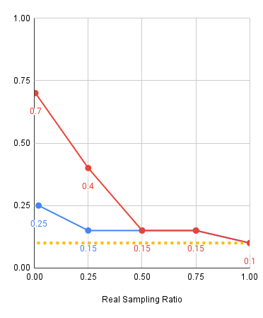
Red: 2000 sim demos, Blue: 500 sim demos, Yellow: Real only baseline
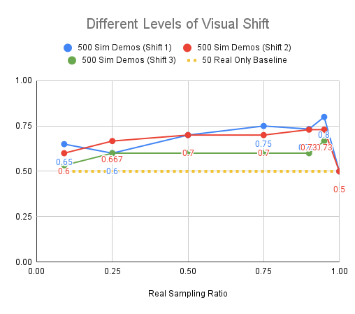
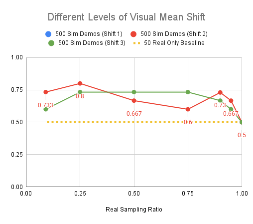
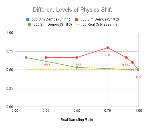
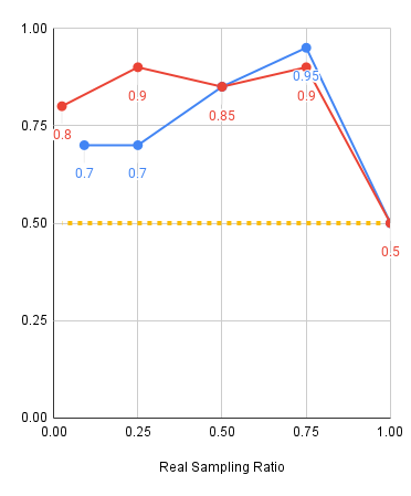
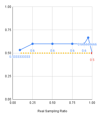
Experiments: Visual Shift
Red: 2000 sim demos, Blue: 500 sim demos, Yellow: Real only baseline
Level 1
Level 2
Level 3
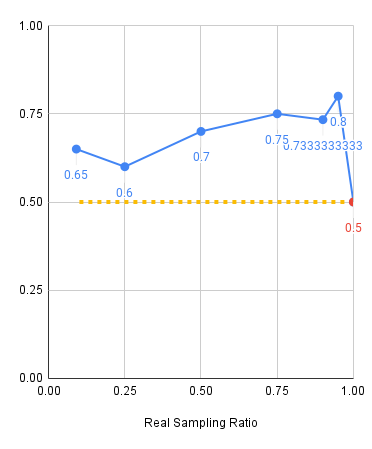
Experiments: Key Takeaways
Mixing ratio takeaways:
- Policy performance is sensitive to alpha, especially in low data regime
- Smaller real dataset => smaller alpha
- Larger real dataset => larger alpha
- If there is sufficient real data, sim data will not help. It also isn't detrimental:
Scaling up sim data:
- Improves model performance at almost all mixtures
- Drastically improves model performance when real data is scarce
- Reduces sensitivity to the mixture ratio when data is plentiful
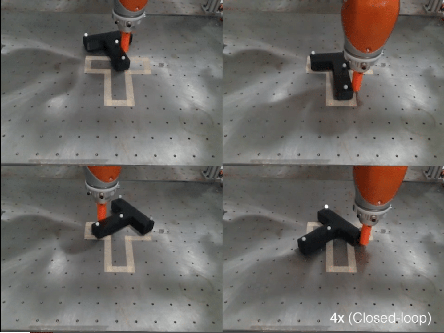
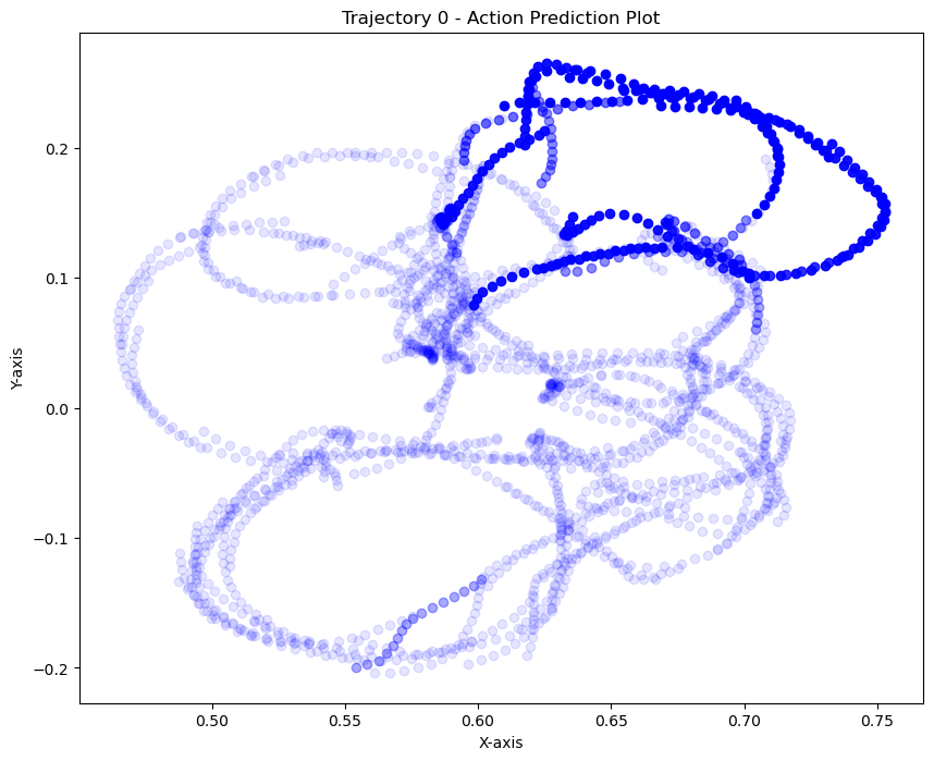
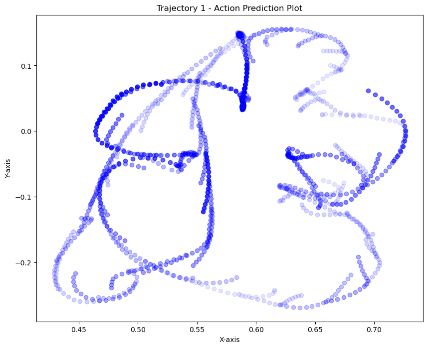
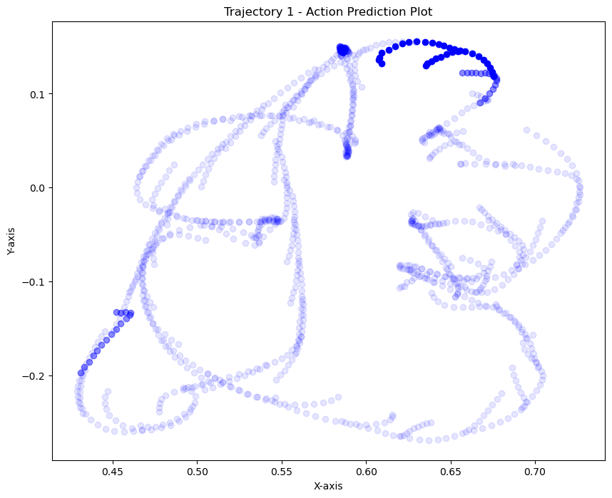
Observation
Cotrained policies exhibit similar characteristics to the real-world expert regardless of the mixing ratio.
- Show the videos...
How does the simulate data help the final policy?
Real vs Sim Data Characteristics
Text
Real Data
- Aligns orientation, then translation
- Sliding contacts
- Leverage "nook" of T
- Larger workspace of initial conditions
Sim Data
- Aligns orientation and translation simultaneously
- Sticking contacts contacts
- Pushes on the short side of the top of T
- Smaller workspace of initial conditions
Hypothesis
1. Cotrained policies rely on real data for high-level decisions. Sim data helps fill in missing gaps.
2. The conditional distributions for real and sim are different (which the model successfully learns).
3. Sim data contains more information about high-probability actions, p(A)
4. Sim data prevents overfitting to real.
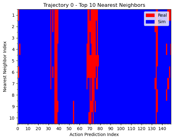
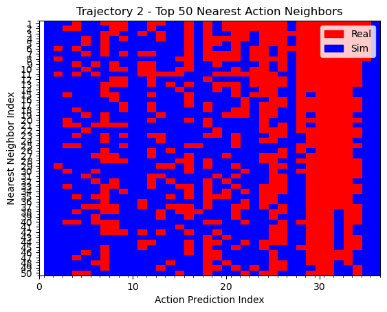
Hypothesis 1
1. Cotrained policies rely on real data for high-level decisions. Sim data helps fill in missing gaps.
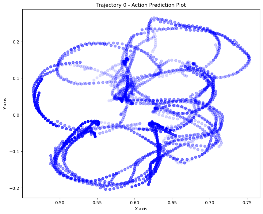
kNN on actions
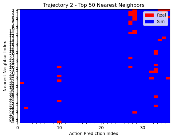
Hypothesis 1
kNN on observation embeddings TODO: change to red
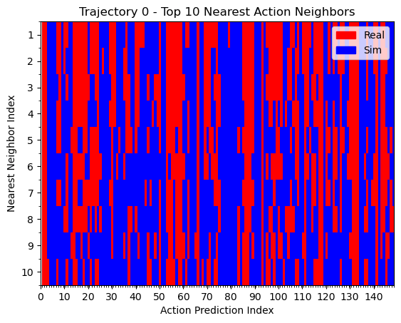
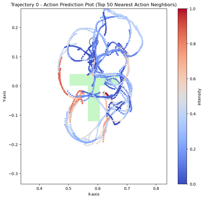
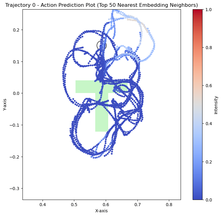
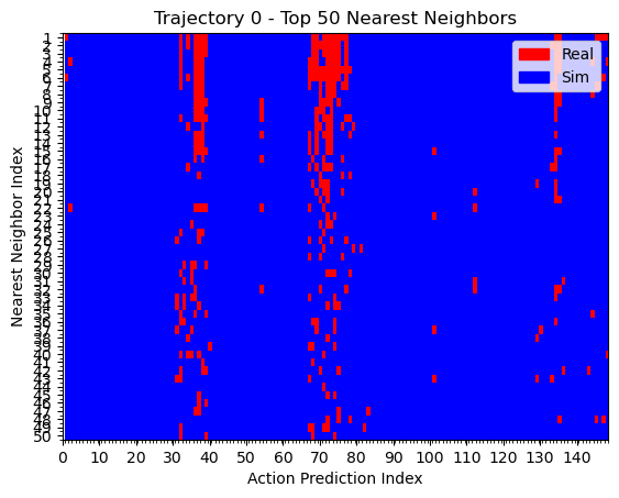
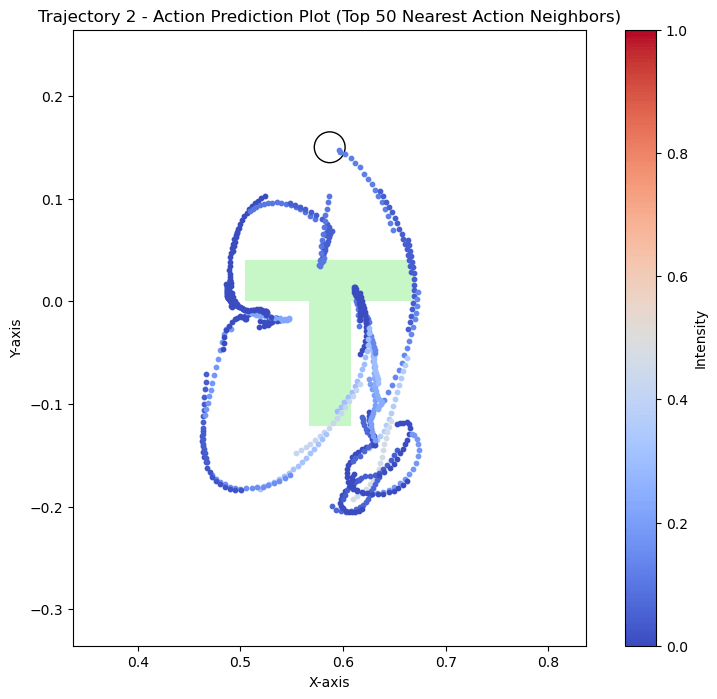
Hypothesis 1
kNN on actions

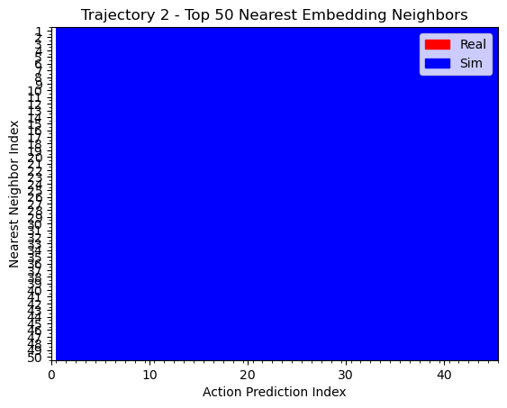
Hypothesis 1
kNN on observation embeddings
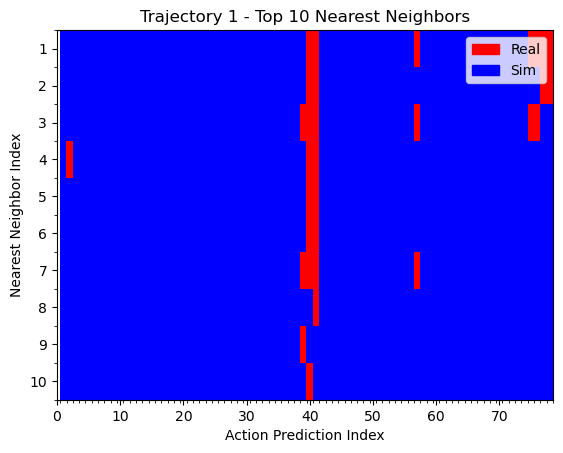
Hypothesis 1
Note to self:
We can see that the policy is closer to real data when the T is far from the goal. During eval, the T is also placed far from the goal. This could explain why the policy appears to use real data for high-level logical decisions: the initial conditions are outside the support of the sim data, so the policy must rely on real world data to make the initial logical decisions
Hypothesis 1
1. Cotrained policies rely on real data for high-level decisions. Sim data helps fill in missing gaps.
kNN on actions

Hypothesis 1
kNN on obs embedding
Hypothesis 1
kNN on actions

Hypothesis 1
kNN on obs embeddings

Hypothesis 1
kNN on actions

Hypothesis 1
kNN on obs embeddings

Hypothesis 2
2. The conditional distributions for real and sim are different which the model successfully learns.
Experiment: roll out the cotrained policy in sim and observe the behavior.
- Show meshcat replays...
- Hard to say if it looks more like real or sim
To-do: need a way to visualize or compare how similar a trajectory is to sim vs real
Hypothesis 3
3. Sim data contains information about high-probability actions (i.e. co-training can help the model learn p(A) )
Future experiment: Cotrain with classifier-free guidance.
- Use real sim data to get more unconditional data from
- Train the conditional model only on
- Sample via classifier free guidance:
Conditional Score Estimate
Unconditional Score Estimate
Immediate experiment: Replace the sim images with all zeros and cotrain.
Hypothesis 4
4. Sim data helps prevent overfitting (acts like a regularizer)