Spatial structure of chromatin: features calling
Aleksandra Galitsyna
“Analysis of omics data” course
Skoltech Term 4
27 April 2020

This presentation can be found at https://slides.com/agalicina/epigenetics-practice4-2020
Notes on EpiPract1
For EpiPract 1, we obtained a bigWig file with the coverage in your experiments:
We may need these files for the last practice on data association (EpiPract5). You can exchange these files with three of your colleagues in any preferable way (e.g. e-mail or copying from the folder on cluster).
For your convenience, I've created the folder for exchange:
Feel free to copy your file to this directory and use other files from there.
$ mv <file.genomecov.bw> <YOUR_CELL_LINE-CHROMOSOME.bw>$ cp ${your_file} /home/shared/EpiPract1/Chromatin spatial structure
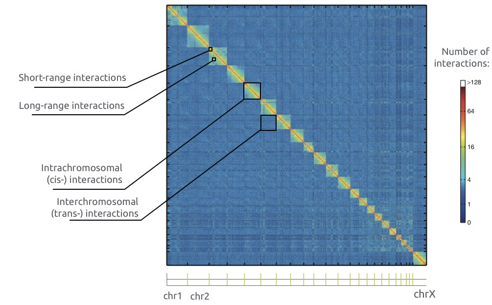
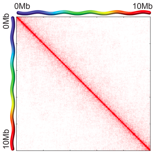
Adopted from Imakaev et al. Nature Methods 2012
Chromosome territories: trans contacts
Bonev et al. Nature Reviews 2016
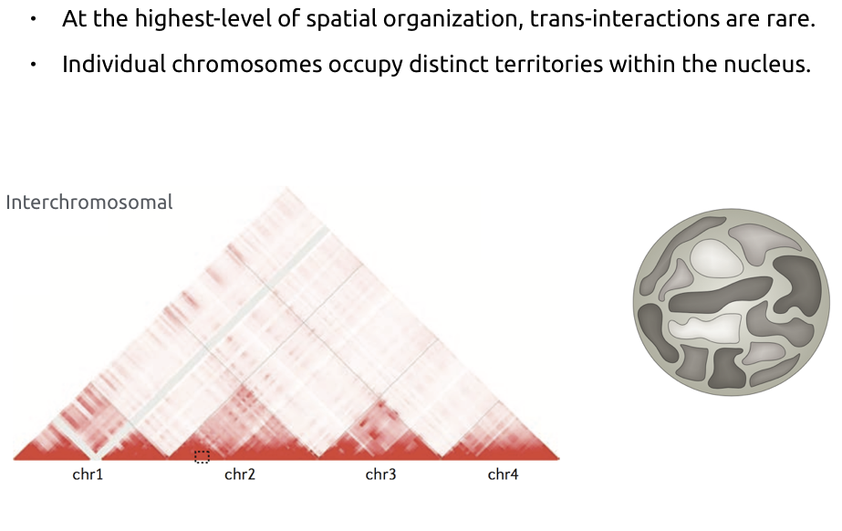
Chromosome territories
Falk et al. Nature 2019
b. Average number of contacts between pairs of chromosomes. Average cis contacts are much higher than trans contacts.
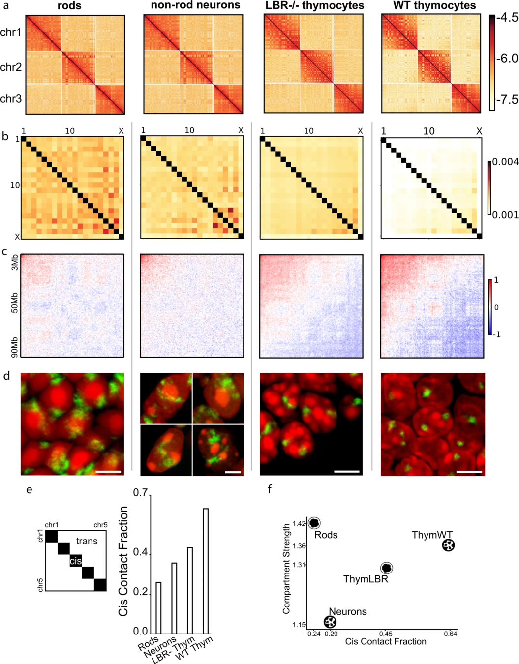
a. Hi-C maps for chr 1, 2, 3 demonstrating territoriality:
Scaling plots: the feature of cis maps
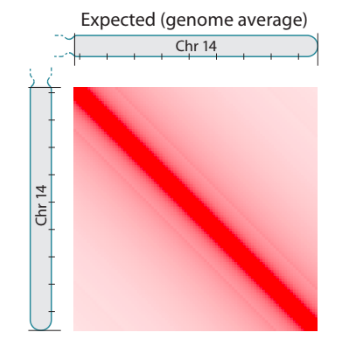
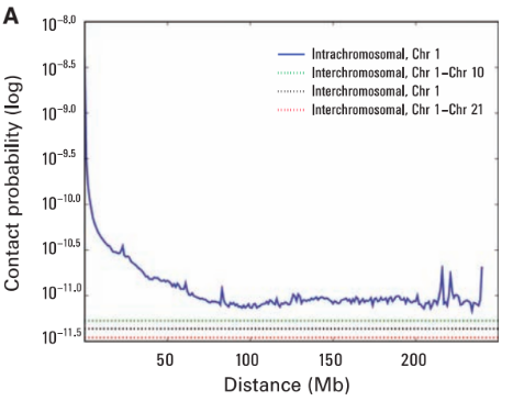
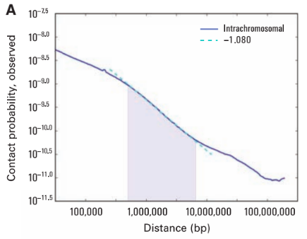
Lieberman-Aiden, 2009
Compartments of chromatin
Bonev et al. Nature Reviews 2016
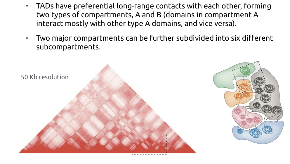
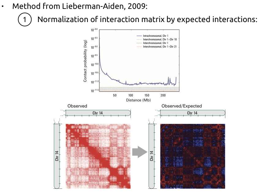
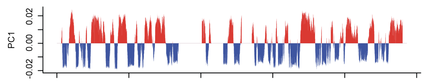
Compartments calling
Lieberman-Aiden et al. Nature 2009
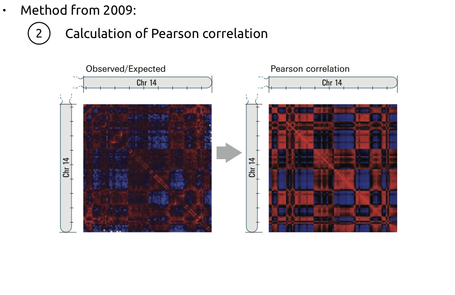
Compartments calling
Lieberman-Aiden et al. Nature 2009
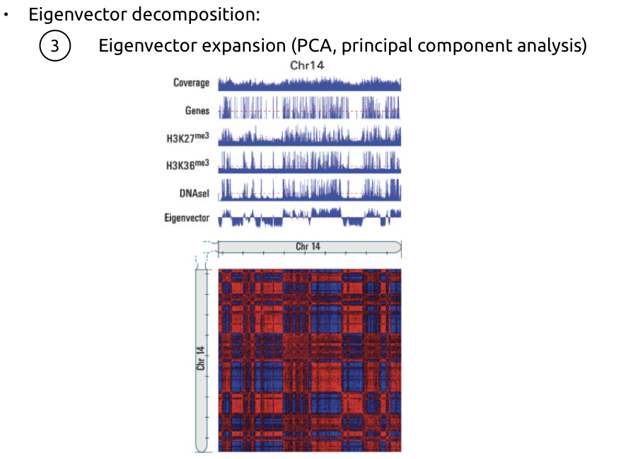
Compartments calling
Lieberman-Aiden et al. Nature 2009
Compartments of chromatin
Falk et al. Nature 2019
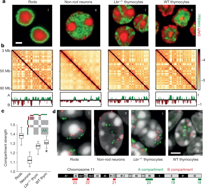
Usual scenario: euchromatin resides in the interior, heretochromatin is outside. On comparison with Hi-C, you see the compartments have different strength:
Compartments of chromatin
Falk et al. Nature 2019
Non-typical scenario, inverted nuclei when the euchromatin is peripheral:
inverted
inverted
usual
Note that compartments on Hi-C are the same for two fundamentally different structures of thymocytes nuclei.
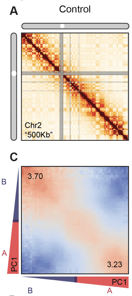
Estimation of compartment strength
Procedure:
1. Call compartments.
2. Calculate observed over expected for Hi-C,
3. Reorder Hi-C rows and columns by the 1st component of PCA,
4. Average neighbouring pixels.
TADs
Bonev et al. Nature Reviews 2016
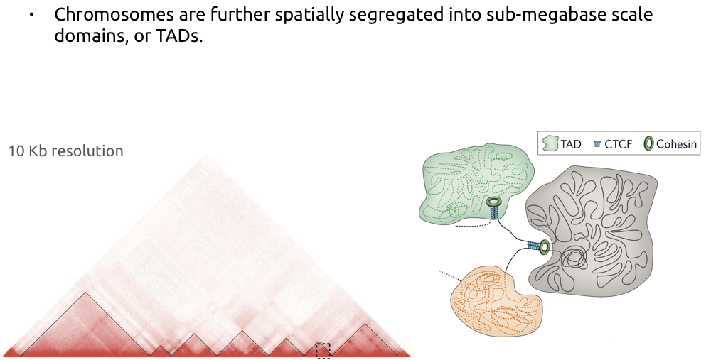
TADs
Filippova et al. Algorithms for Molecular Biology 2014
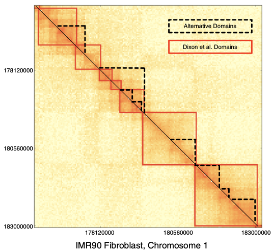
TADs are hierarchical, there is no single solution for the TAD calling problem:
- Armatus is one of the programs trying to solve this problem.
- Armatus is based on a dynamic programming algorithm that has an adjustable parameter.
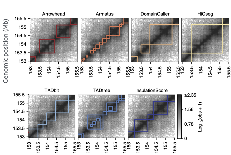
TADs callers comparison
Forcato et al. Nature Methods 2017
TADs callers comparison
based on Crane, 2015
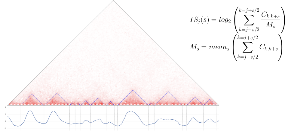
- Insulation score - is one of the simplest algorithms for TADs search:
- Calculate Insulation score for each genomic bin,
- Look for the local minima:
Loops of chromatin
Bonev et al. Nature Reviews 2016
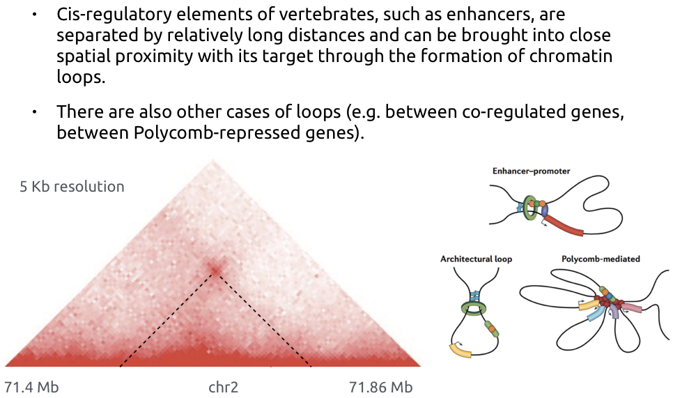
Loops of chromatin
Bonev et al. Nature Reviews 2016
Different names for the same feature:
- loops
- dots,
- enriched contacts
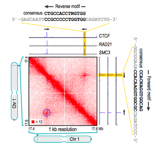
Properties of loops in mammals
Rao et al. Cell 2014
In mammals, loops are associated with CTCF binding motif with a particular type of orientation:
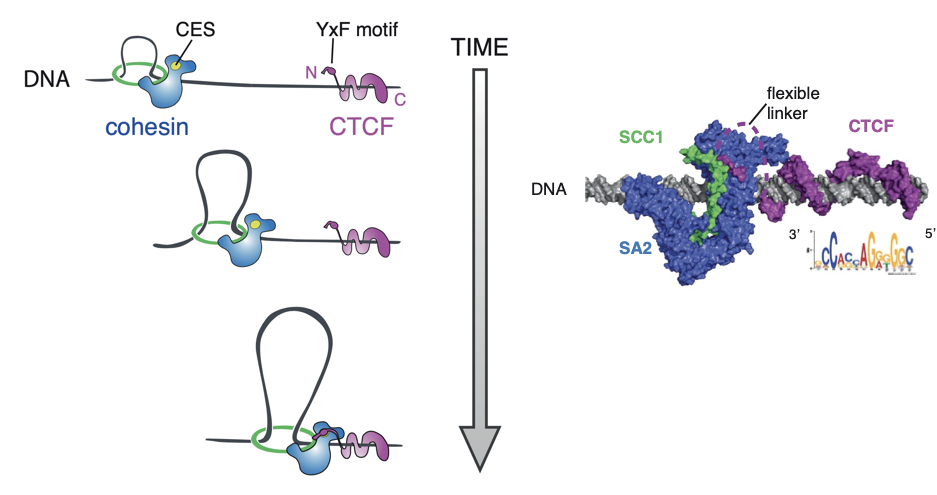
Properties of loops in mammals
Li et al. Nature 2020
Mechanism of loop extrusion as an explanation of formation of bright dots:
Properties of loops in mammals
Properties of loops in mammals
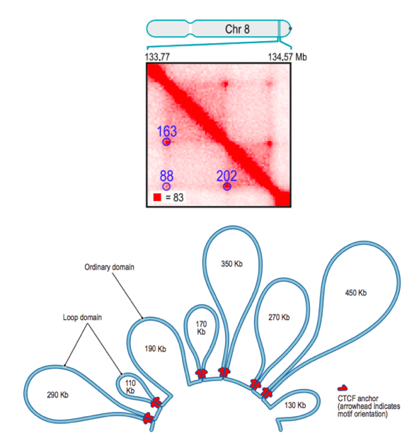
Rao et al. Cell 2014
Due to this mechanism, dots are also hierarchical:
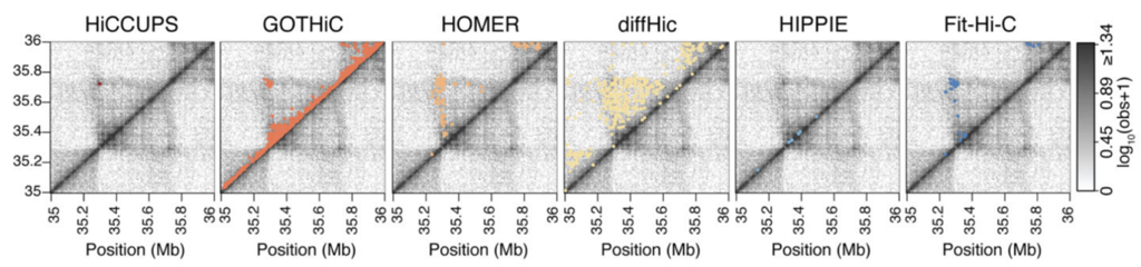
Loops calling algorithms
Forcato et al. Nature Methods 2017
There is a variety of tools for calculation of enriched contacts in Hi-C, but not all of the results can be considered loops:
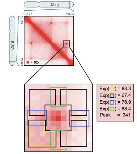
Loops calling algorithm: HiCCUPS
Rao et al. Cell 2014
Hi-C Computational Unbiased Peak Search:
Average loop plot
Flyamer Bioinformatics 2019
We can average Hi-C plots around all the pixels of the found loops:
https://github.com/Phlya/coolpuppy

Practice:
Features calling on Hi-C
In this practice:
We'll need conda environment "hic" (see instructions on activation can be found in EpiPract3). We will:
- Plot P(s), or scaling plots
- Call compartments, create saddle plot
- Call TADs and plot them
For two organisms:
For Drosophila Hug 2017: you may use your cool files obtained for EpiPract3 (*), but it's not required.
Working with mcool files
.mcool is a multi-resolution cool file for Hi-C data storage.
Copy these files to your current folder:
- /home/galitsyna/EpiPract4/cool/GM12878_Rao2014.hg19.1000.mcool
- /home/galitsyna/EpiPract4/cool/S2_Wang2017.dm3.100.mcool
-
the dataset on embryogenesis from the previous practice. If you do not have your own file, feel free to use the one with your prefix from the same folder /home/galitsyna/EpiPract4/cool/
The files are already merged by technical replicates to increase coverage.
You can check what resolutions are available for your mcool-file:
Then you can get detailed information about your single-resolution cooler (let's stick to 10 Kb resolution throughout this practice):
Note that you access different cooler resolutions by this query: ${cool}::/resolutions/10000
$ cooler ls GM12878_Rao2014.hg19.1000.mcool$ cooler info GM12878_Rao2014.hg19.1000.mcool::/resolutions/10000"Scaling plots"
Let's plot the dependence of contact probability from the genomic distance with HiCExplorer for Drosophila set.
The basic command for 10 Kb-resolution looks as follows:
However, we need also to:
- add both Drosophila cool files (S2 from Wang and your own on embryogenesis) at the same resolution (10 or 20 Kb),
- add appropriate --labels to the plot,
- skip the diagonal (remember Hi-C artifacts from last lesson?).
$ hicPlotDistVsCounts --matrices ${file.mcool}::/resolutions/10000 --plotFile ${output.png}Task 1 (1 point): Write down the final command that you've got. Explain briefly what it does and why you need queries/parameters.
Task 2 (1 point): Add the resulting plot to your report. What is the difference between two datasets? What are possibly due to technical and what are due to biological reasons?
"Scaling plots"
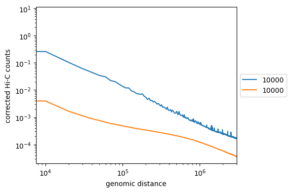
Non-optimized example, similar to what you should get:
Text
Labels need to be corrected
Note the intercept in the beginning. It corresponds to contact probability at the smallest distance. Does it depend on coverage?
Do we get a strict line? If not, it might indicate more frequent/rare short- or long-distance contacts.
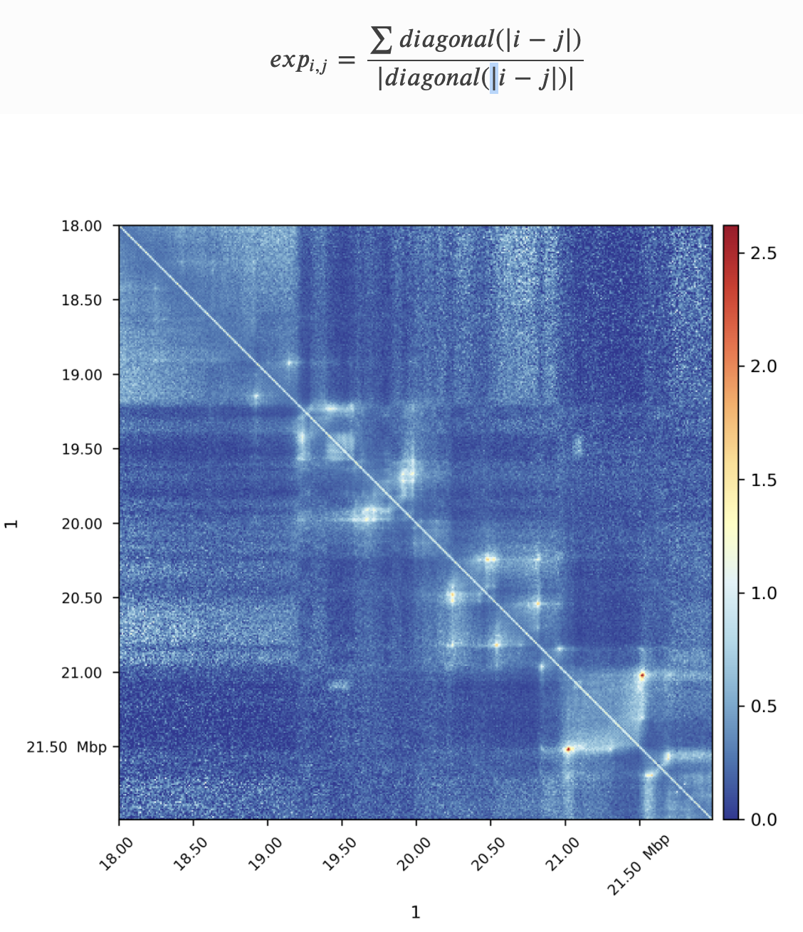
Plotting observed over expected
We will use HiCExplorer's hiCTransform and hiCPlotMatrix for plotting the observed over expected:
We will need to modify in these commands:
- Compute expected for a single chromosome with --chromosome chr1, or for each chromosome independently with --perChromosome (to reduce computation time).
- For plotting, clear the bins that have poor coverage (option --clearMaskedBins)
- Specify the region to plot (--region option). Let's take 10 Mb-resion and compare between Drosophila and human. For Drosophila use chr2L:0-10000000 and chr1:0-10000000 for human.
- Rescale the heatmap of the plot to --vMin 0, --vMax 2.5.
$ hicTransform --matrix ${file.mcool}::/resolutions/10000 --outFileName ${normalized.cool} --method obs_exp
$ hicPlotMatrix -m ${normalized.cool} -o ${output.png}
Task 3 (1 point): Add the resulting commands and plots with expected maps for 10 Mb-regions of S2 Drosophila and GM12878 human data to your report. What features can you observe on this plot? Are they present in both species? Do they have the same prominence and size in genomic units?
Task 4 (1 point*): Plot the same region for Drosophila embryogenesis dataset. What differences do you observe with S2 cell line? What might be explained by technical reasons and what by biological? Consult with the paper.
Calling compartments
For this task, we will use cooltools Command Line Interface (CLI).
Compartments call can be divided into following steps:
-
Computing expected:
- Call compartments:
- Plot saddle plot:
! Note that we don't do phasing of compartments, so we don't know what is actually A and what is B.
Task 5 (2 point): Run for both Drosophila and human. Try -n 10 and 20. What are your conclusions?
Are both compartments strong for both species?
$ cooltools call-compartments ${file.mcool}::/resolutions/10000 -o ${compartments.tsv} --contact-type trans$ cooltools compute-expected ${file.mcool}::/resolutions/10000 -o ${expected.tsv}$ cooltools compute-saddle ${file.mcool}::/resolutions/10000 ${compartment.tsv}.trans.vecs.tsv ${expected.tsv} -o ${saddle} --fig png -n 10TADs calling
We will use HiCExplorer HiCFindTADs functionality.
1. Call TADs:
2. Convert cool format to h5:
3. Create tracks.ini file (example on the right), with vim on nano.
4. Run plotting step:
Task 6 (2 points*): Read about TAD calling in HiCExplorer. What are other parameters that you can try to vary? Try 5-6 different sets, pick the best and describe your observations.
Task 7 (3 points*). Run the same for human and data on embryogenesis at 10 Kb resolution. Describe your observations.
hicFindTADs --matrix ${file.mcool}::/resolutions/10000 --outPrefix ${tmp.tads} --correctForMultipleTesting fdr --minDepth 30000 --maxDepth 10000000 --step 30000 --numberOfProcessors 2[x-axis]
where = top
[hic matrix]
file = ${converted.file.h5}
title = Hi-C data
depth = 300000
transform = log1p
file_type = hic_matrix
[tads]
file = ${tads.file.domains.bed}
file_type = domains
border_color = black
color = none
overlay_previous = share-y$ hicPlotTADs --tracks track.ini -o {tads.pnf} --region chr2L:0-1000000$ hicConvertFormat --matrices ${file.mcool}::/resolutions/10000 -o ${converted.file.h5}.h5 --inputFormat cool --outputFormat h5tracks.ini
Additional slides:
Applications of chromosome conformation capture
Single-cell Hi-C

Flyamer et al. Nature 2017

Single-cell Hi-C: results of modelling
Stevens et al. Nature 2017

Single-cell Hi-C: data processing
work in preparation
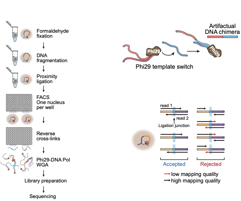
- Wet lab protocol:
- Polymerase creates erroneous contacts:
- Rigorous data filtration protocol
One Read-Based Interactions Annotation (ORBITA):
Single-cell Hi-C: data processing
-
Number of contacts per restriction fragment for two snHi-C approaches:
hiclib as in Flyamer 2017
ORBITA - One Read-Based Interactions Annotation
We expect at most 4 contacts per restriction fragments (2 DNA copies per cell, 2 ends to be ligated)
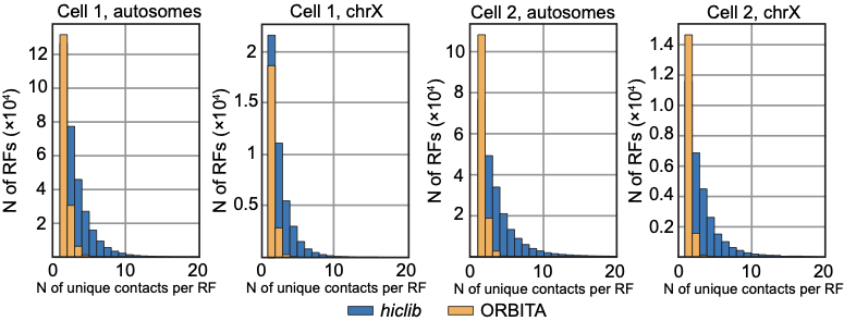
work in preparation
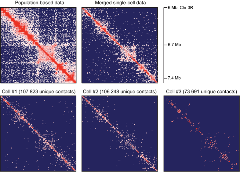
Single-cell Hi-C: data processing
-
Resulting Hi-C datasets for Drosophila melanogaster
work in preparation

Other single-cell Hi-C approaches
-
Barcoding-based protocol:
Ramani et al. Nature methods 2017
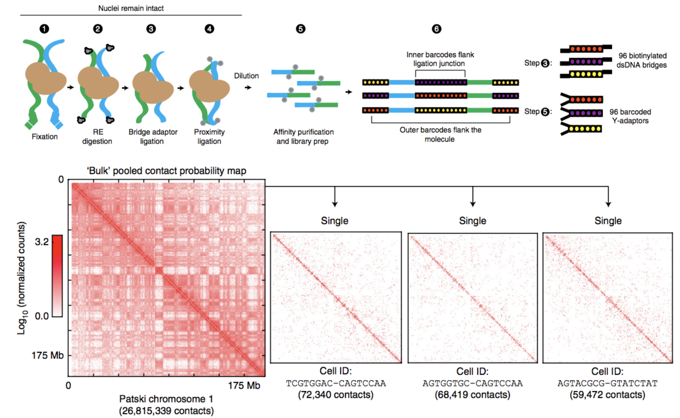
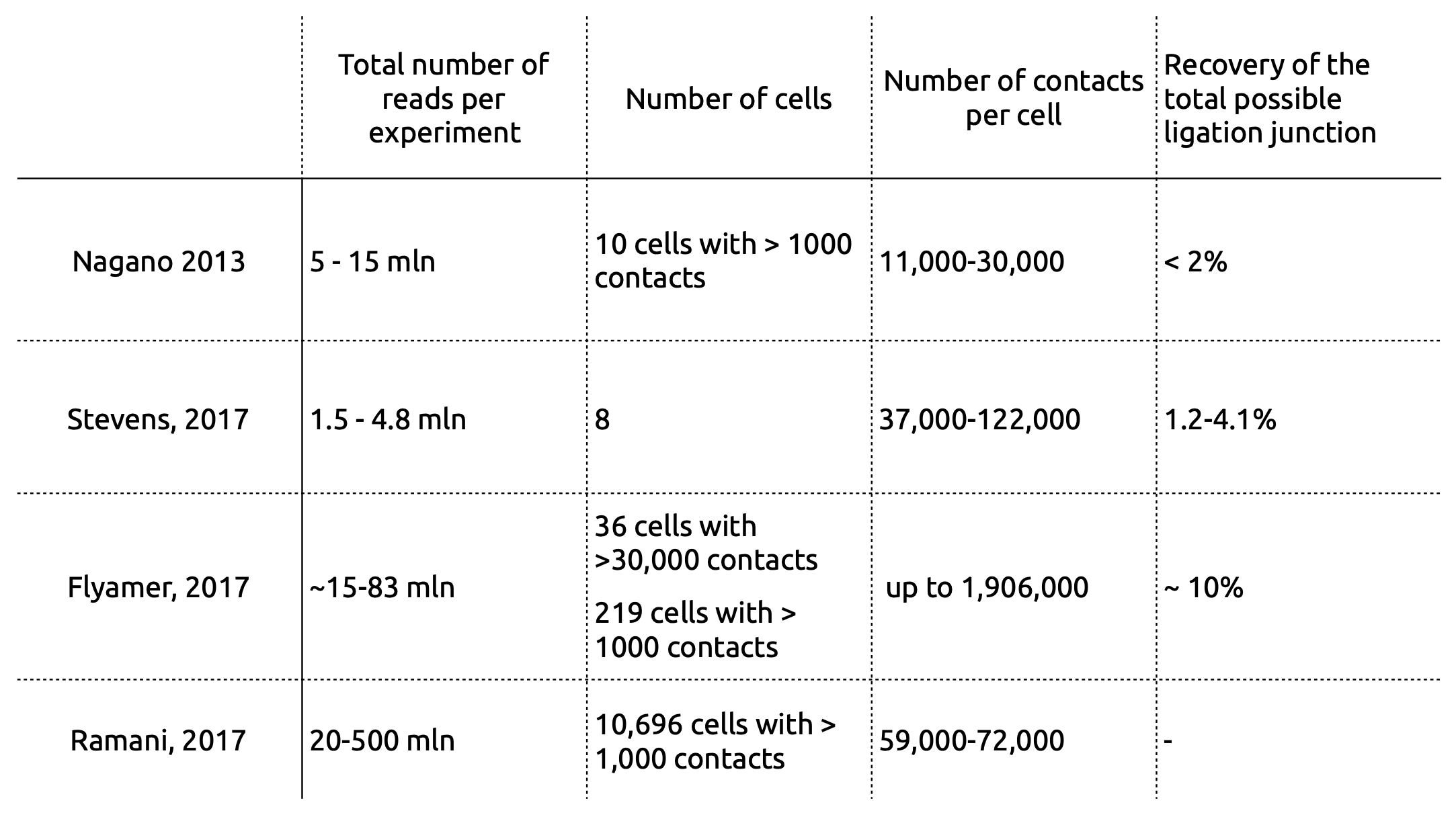
Current limitations of single-cell Hi-C
Ramani et al. Nature methods 2017
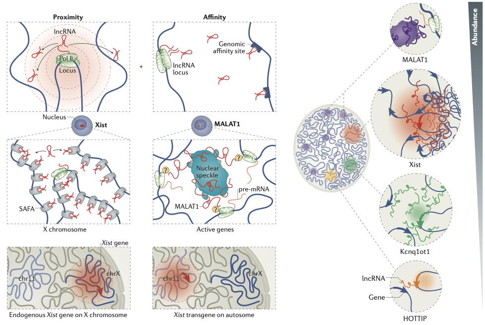
RNA-DNA interactions
Engreitz et al. Nature Reviews 2016
RNA-DNA interactions
Variety of methods exist for RNA-DNA interactome assays:
- Detection of chromatin-associated RNAs:
- Nuclear fractionation - Werner & Ruthenburg 2015
- One-vs-all targeting:
- ChIRP-seq (chromatin isolation by RNA purification) - Chu et al. 2015
- CHART (capture hybridization analysis of RNA targets) - Simon et al. 2011
- RAP (RNA Antisense Purification) - Engreitz et al. 2014
- Many-vs-many targeting:
- GRID-Seq (global RNA interactions with DNA by deep sequencing) - Li et al. 2017
- MARGI (mapping RNA-genome interactions) - Sridhar et al. 2017
- ChAR-Seq (chromatin-associated RNA sequencing) - Bell et al. 2018
- other
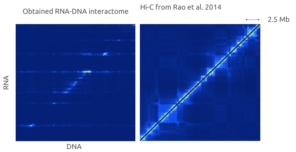
Red-C for RNA-DNA high-throughput assay
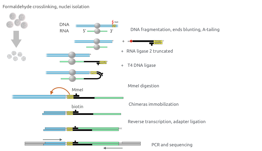
Gavrilov, Zharikova, Mironov, Galitsyna, paper in review
Red-C for RNA-DNA high-throughput assay
Gavrilov, Zharikova, Mironov, Galitsyna, paper in review