Neural Ordinary Differential Equations
Presented by Alex Feng
Ricky T. Q. Chen, Yulia Rubanova, Jesse Bettencourt, David Duvenaud
Outline
- Related Work/Background
- Model Structure
- Experiments
- Continuous Normalizing Flows
- A Generative Latent Function Time-Series Model
- Conclusions
Background
- Recurrent Networks
- LSTM/GRU Blocks
- Residual Blocks
Recurrent Neural Networks
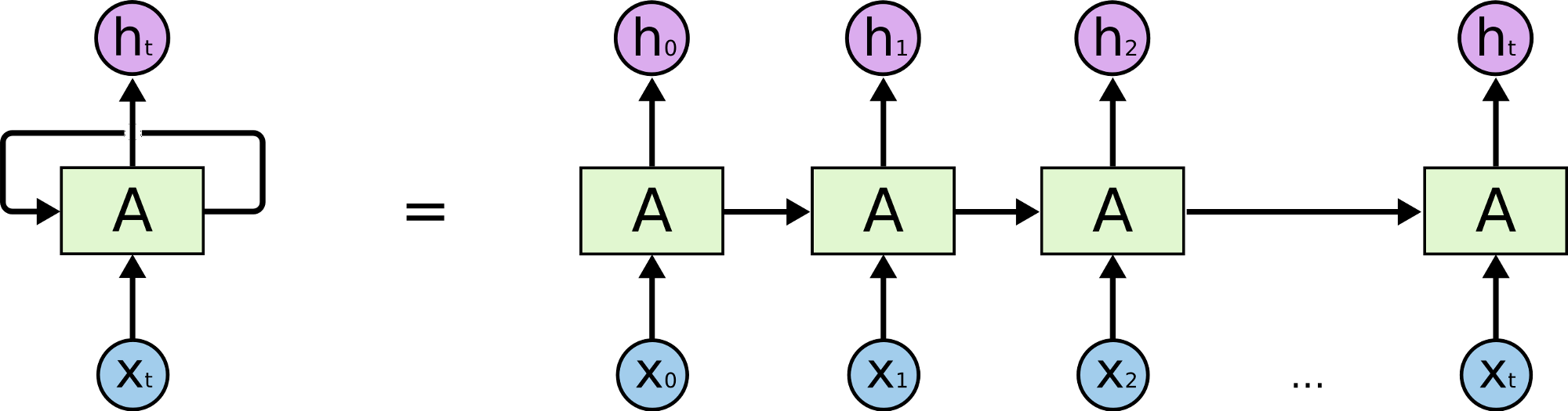
Source: colah's blog
Vanishing Gradient Problem
- Gradients decay exponentially with number of layers
- Becomes impossible to learn correlations between temporally distant events
LSTMs
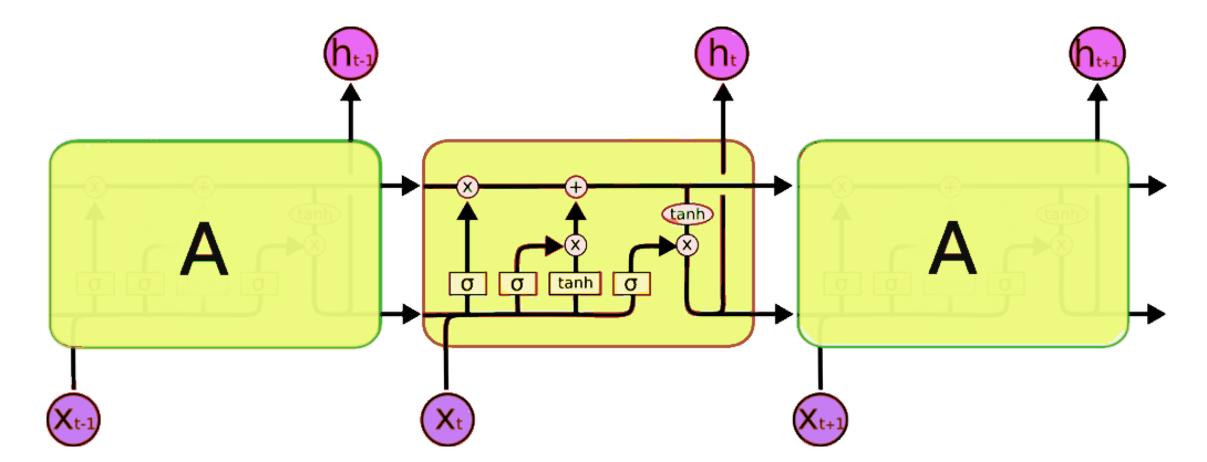
Source: colah's blog
GRUs
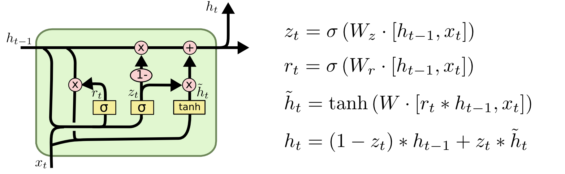
Source: colah's blog
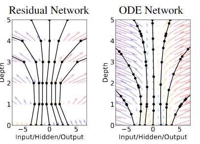
Residual Networks
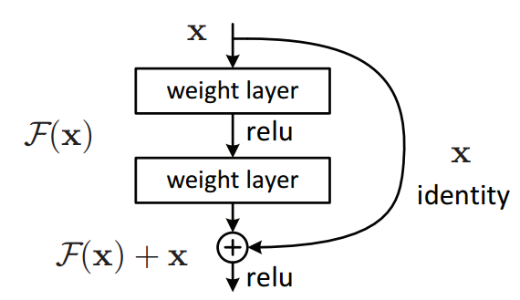
Source: towards data science
Transformations on a Hidden State
$$\pmb h_{t+1}=\pmb h_t+f(\pmb h_t,\theta_t)$$
Euler's Method
$$f(x+h)=f(x)+hf'(x)$$
Ordinary Differential Equations
- Describe the derivative of some function
- Can be solved with a "black box" solver
- $$\pmb h_{t+1}=\pmb h_t+f(\pmb h_t,\theta_t)\rightarrow\frac{d\pmb{h}(t)}{dt}=f(\pmb{h}(t),t,\theta)$$
ODE Solvers
- Runge-Kutta
- Adams
- Implicit vs. Explicit
- Black Box
Updating the Network
- RK Backpropagation
- Adams Method
- Adjoint Method
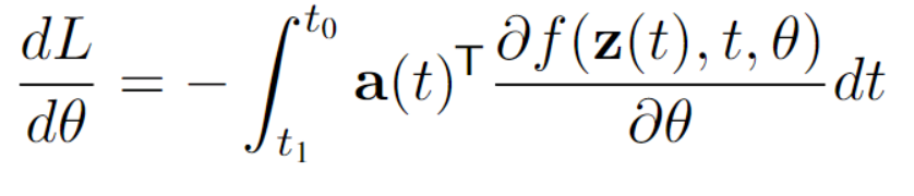
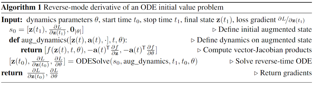
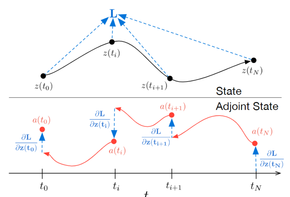
The Adjoint Method
\(L\)(ODESolve(\(\pmb{z}(t_0),f,t_0,t_1,\theta))\)
$$\pmb{a}(t)=\frac{\partial L}{\partial \pmb{z}(t)}$$
$$\frac{d\pmb{a}(t)}{dt}=-\pmb{a}(t)^T\frac{\partial f(\pmb{z}(t),t,\theta)}{\partial\pmb{z}}$$
Results in Supervised Learning
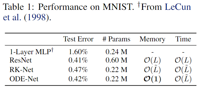
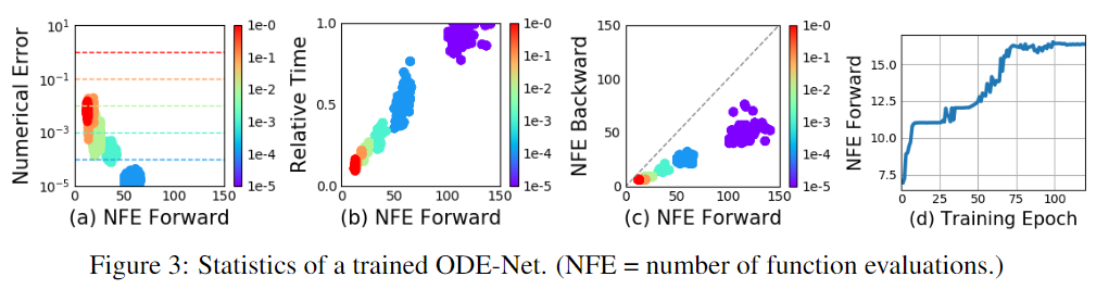
Error Control
Normalizing Flows
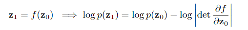

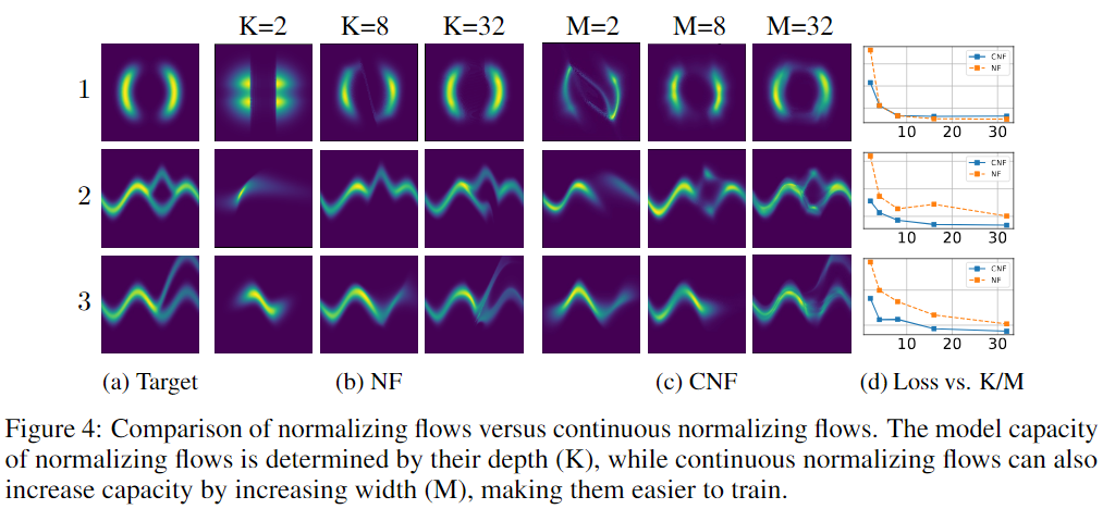
Continuous Normalizing Flows
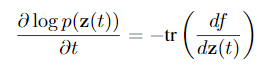
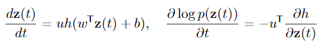

Multiple Hidden Units
\frac{dz}{dt}=\Sigma_n \sigma_n(t) f_n(\pmb z)
Experiments in CNFs
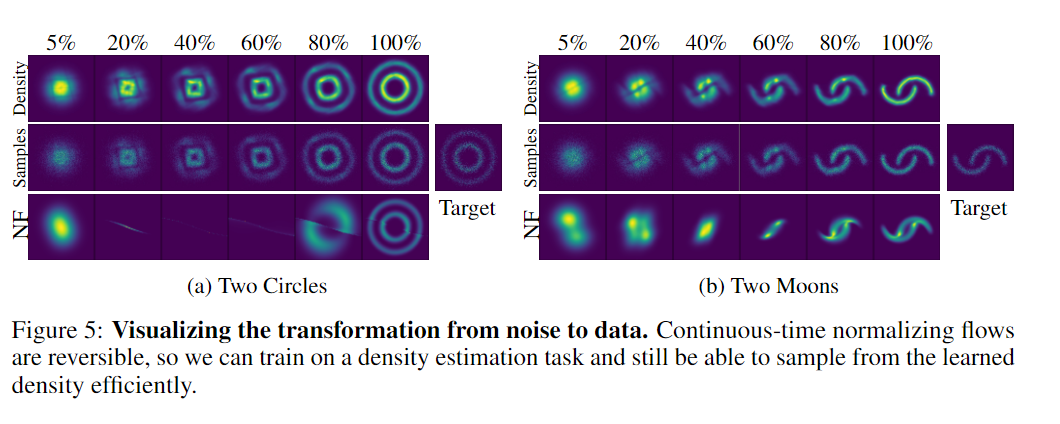
Maximum Likelihood Training
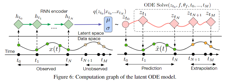
A Generative Latent Function Time-series Model
- Applying neural networks to irregularly sampled data is difficult
- Typically observations are put into bins of fixed duration, but this leads to missing data issues
- Each time-series is represented by a latent trajectory
- Each of these is determined by a local initial state \(\pmb z_0\) and a global set of dynamics
- Given a set of times, an ODE solver produces a set of latent states at each observation

Training the Model
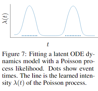
Poisson Process Likelihoods
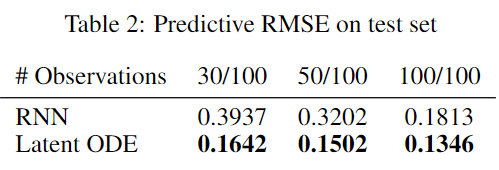
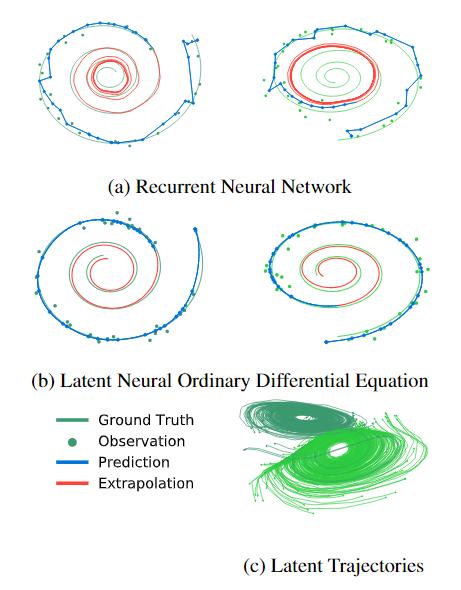
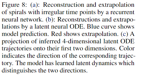
Experiments
Limitations
- Minibatching more complicated
- Requires Lipschitz nonlinearities such as tanh or relu
- User must choose error tolerances
Conclusions
- Adaptive evaluation
- Tradeoff between speed and accuracy
- Applications in time-series, supervised learning, and continuous normalizing flows
Future Work
- Regularizing ODE nets to be faster to solve
- Getting the time-series model to scale up and extend it to stochastic differential equations.
- CNFs as a practical generative density model
Closing Remarks
- Some figures were hard to understand at first
- Lacks comparison to state-of-the-art
- Overall mainly a proof-of-concept paper