Machine Learning
Tools and Practices...
Machine Learning
Tools and Practices...
and Concepts...
and whatever I'll have time for in 25 minutes
So, what is Machine Learning?
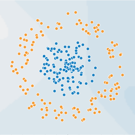
First, you have data
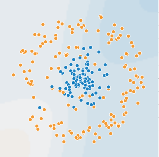
... it's more like this, in fact
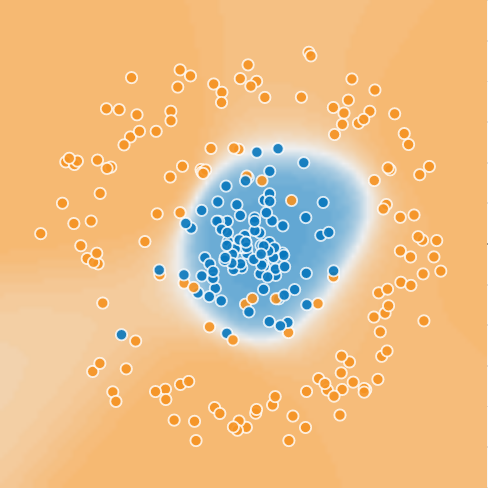
And then, you have a model that discriminates
OK, then how is Machine Learning done?
Conceptually
- Clean data
- Clean data
- and ... clean data
- ...
Conceptually
- ...
- Ask domain experts for to develop new features
- Make your model (a simple one first)
- Profit OR get a better model/new data + clean data
And now the meat!!
The Holly Quaternity
Pandas
import pandas as pd

data = pd.read_csv("dataset/somedataset.csv") # or a lot of other file formats

no_nans_data = data.fillna(0)

no_nans_data["new_feature"] = some_data_transformation(no_nans_data["old_feature1"],
                                                       no_nans_data["old_feature2"])

# ... some more data wrangling here

labels = final_data.pop("label").values
features = final_data.values

# and a lot of other stuff, like pivot tables, sampling, plotting
# think of Pandas as Excel with a Python API... only Python API
# Pandas is used in the initial phase of the machine learning workflow
Scikit-Learn
from sklearn import linear_model, decomposition, datasets
from sklearn.pipeline import Pipeline
from sklearn.model_selection import GridSearchCV

logistic = linear_model.LogisticRegression()
pca = decomposition.PCA()

pipeline = Pipeline(steps=[('pca', pca), ('logistic', logistic)])

pca.fit(features)

# Prediction
n_components = [20, 40, 64]
Cs = np.logspace(-4, 4, 3)

# Parameters of pipelines can be set using ‘__’ separated parameter names:
estimator = GridSearchCV(pipeline,
                         dict(pca__n_components=n_components,
                              logistic__C=Cs))
estimator.fit(features, labels)
Matplotlib
import matplotlib.pyplot as plt
plt.figure(1, figsize=(4, 3))
plt.clf()
plt.axes([.2, .2, .7, .7])
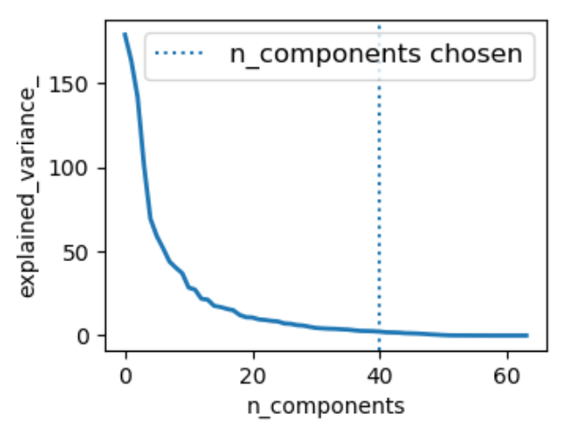
plt.plot(pca.explained_variance_, linewidth=2)
plt.axis('tight')
plt.xlabel('n_components')
plt.ylabel('explained_variance_')
plt.axvline(estimator \
.best_estimator_ \
.named_steps['pca'] \
.n_components,
linestyle=':',
label='n_components chosen')
plt.legend(prop=dict(size=12))
plt.show()
Numpy (sometimes)
Thank you!
questions?
Links to get you started
- pandas.pydata.org/pandas-docs/stable/10min.html
- scikit-learn.org/stable/tutorial/index.html
- matplotlib.org/users/pyplot_tutorial.html