DIVE INTO
Artificial Neural Networks
Alireza Afzal Aghaei
M.Sc student at SBU
Overview
- Introduction
- Biological neural networks
- Neuron
- Artificial neural networks
- Backpropagation
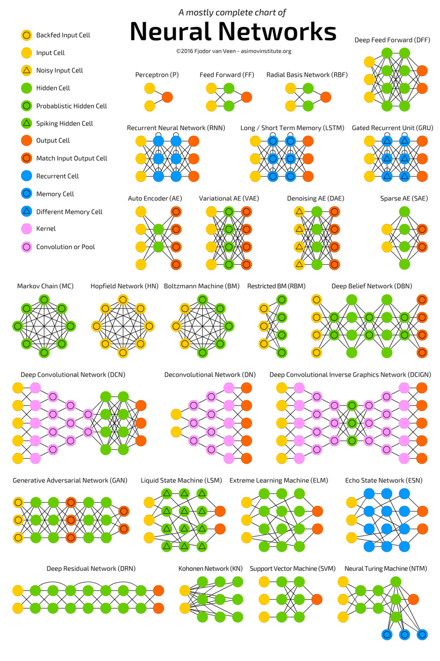
- Other types of ANN
- CNN
- RNN
- LSTM
- Some Examples
Types of learning
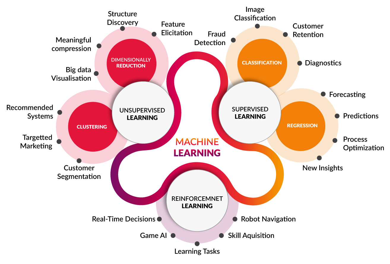
Types of learning
offline learning vs online learning
The motivation of studies in neural networks lies in the flexibility and power of information processing that conventional computing machines do not have
Motivation
Whats ANN?
- Artificial Neural Network is an information-processing system that has certain performance characteristics in common with biological neural networks
- It have been developed as generalizations of mathematical models of human cognition or neural biology
How it works?
Information processing occurs at many simple elements called neurons.
How it works?
- Signals are passed between neurons over connection links
- Each connection link has an associated weight
- Each neuron applies an activation function to its net input
- Each neuron returns new output signal
Biological Neural Networks
LET'S DIVE INTO BIOLOGY
nEURON
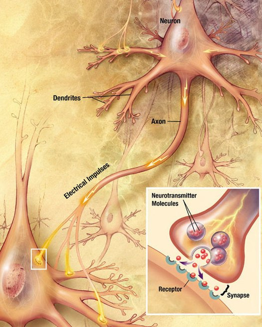
A neuron, is an electrically excitable cell that receives, processes, and transmits information through electrical and chemical signals
nEURON
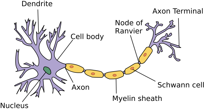
nEURON Structure
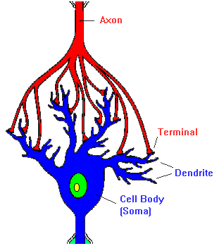
- Dendrites
- Soma
- Axon
Dendrites
- Tree-like structure
- Receives signal from surrounding neurons
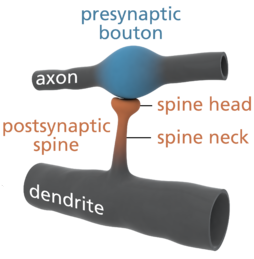
- Dendritic spine: increase the surface area of the dendrite to receive more information
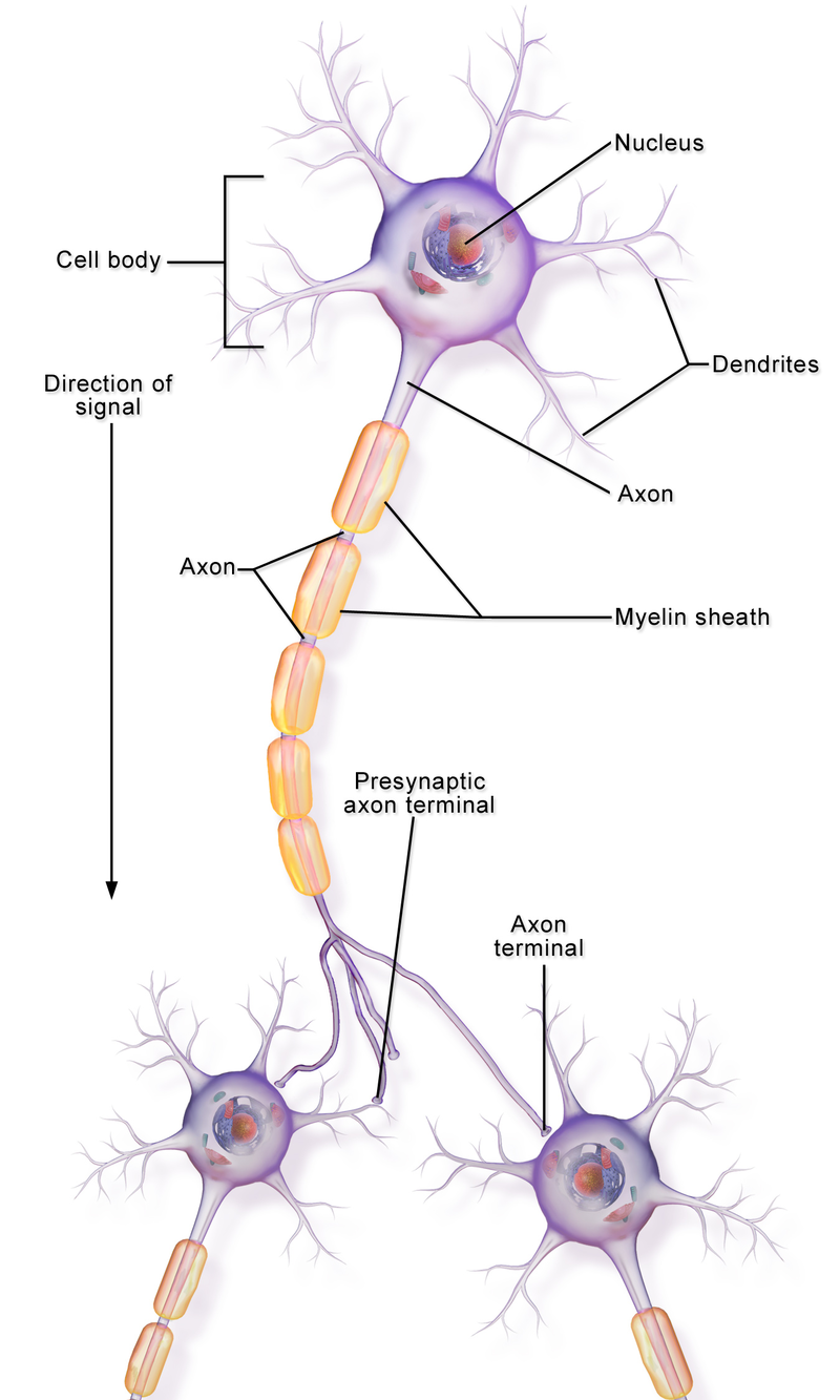
Axon & Myelin
- Axon is a thin cylinder that transmits the signal from one neuron to others.
- Myelin insulates nerve cell axons to increase the speed at which signal travels from one nerve cell body to another

SYNAPSE
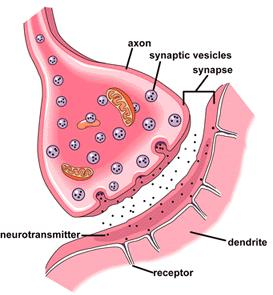
- Gaps between two neuron
- Synaptic plasticity
- Synapse's strength may be modified by experience
excitation & inhibition
- Excitatory signaling from one cell to the next makes the latter cell more likely to fire
- Inhibitory signaling makes the latter cell less likely to fire
Hebb Rule
the connection between the two neurons is strengthened when both neurons are active at the same time
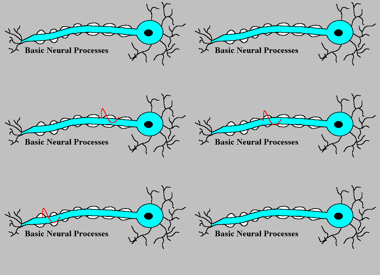
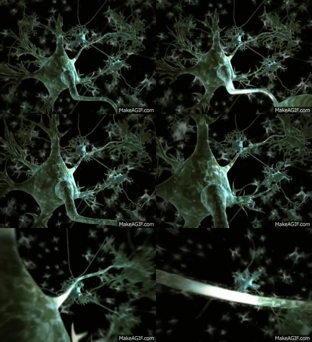
neuron signal transmission
Other kind of neurons
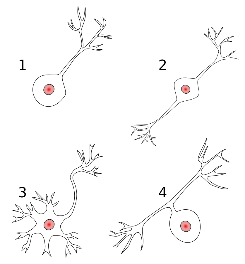
- Unipolar
- Bipolar
- Multipolar
- Pseudounipolar
Summary
-
Dendrite: It receives signals from other neurons
-
Soma: It sums all the incoming signals to generate input
-
Axon: When the sum reaches a threshold value, neuron fires
-
Synapses: The point of interconnection of one neuron with other neurons
-
The connections can be inhibitory or excitatory in nature
-
Hebb rule
Summary
So, neural network, is a highly interconnected network of billions of neuron with trillion of interconnections between them
Further reading
Artificial Neural Networks
LET'S DIVE INTO ARTIFICIAL NEURAL NETWORKS
Analogy of ANN with BNN
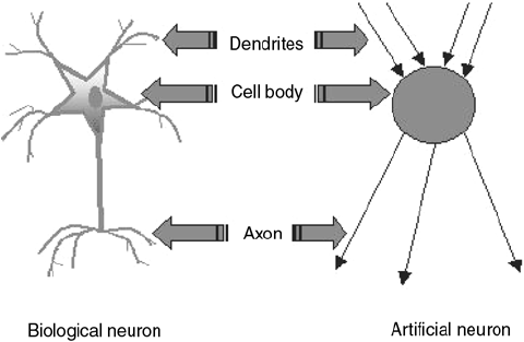
ANALOGY OF ANN WITH BNN
| Criteria | BNN | ANN |
|---|---|---|
| Processing | Massively parallel, slow
|
Massively parallel, fast but inferior than BNN |
| Size | 10 11 neurons and 10 15 interconnections | Depends |
| Learning | Tolerate ambiguity | Precise |
| Fault tolerance | robust | Performance degrades with partial damage |
| Storage | synapse | Continuous memory |
Artificial Neuron Structure
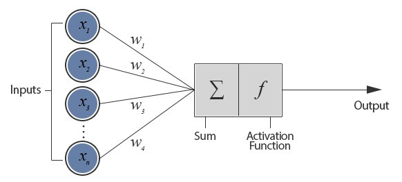
we call this artificial neuron perceptron
ARTIFICIAL NEURon STRUCTURE
- Weight represents the strength of the interconnection
- Sum corresponds to any numerical value from 0 to infinity
- Threshold is set to limit the response to arrive at desired value
ACTIVATION FUNCTIONS
Can we use any arbitrary activation function?
- continuos
- differentiable
- monotonically non-decreasing
- derivative should be easy to compute
Activation functions: Identity
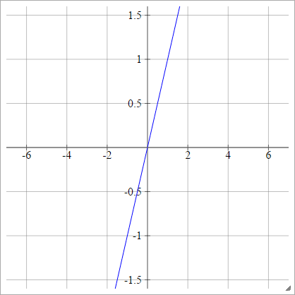
- Bad idea!
Activation functions: step
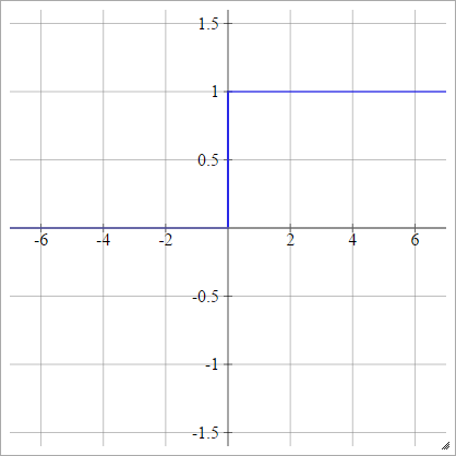
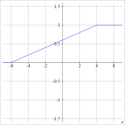
Activation functions: Piecewise Linear
Activation functions: Sigmoid
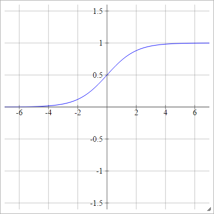
Activation functions: Piecewise Linear
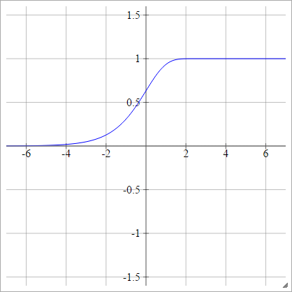
Activation functions: Bipolar
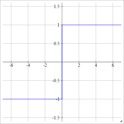
Activation functions: Bipolar Sigmoid
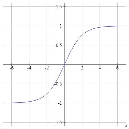
Activation functions: Tanh
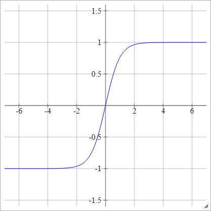
Activation functions: LeCun's Tanh
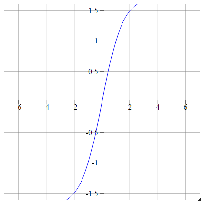
Activation functions: Hard Tanh
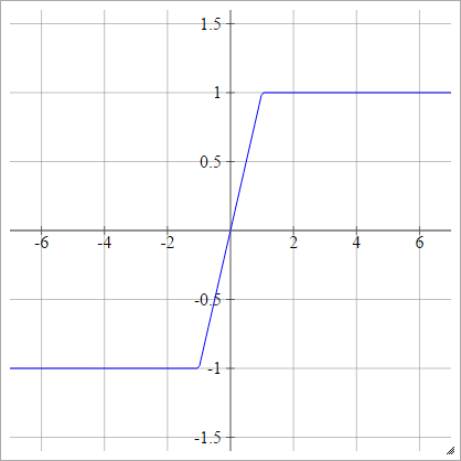
Activation functions: Absolute
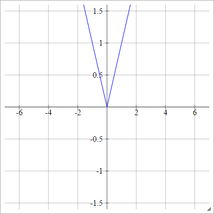
Activation functions: Relu
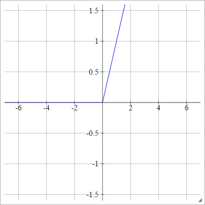
Why ReLU is Non linear?
Activation functions: Leaky ReLU
For negative X the gradient go towards 0 so the weights will not get adjusted during gradient descent
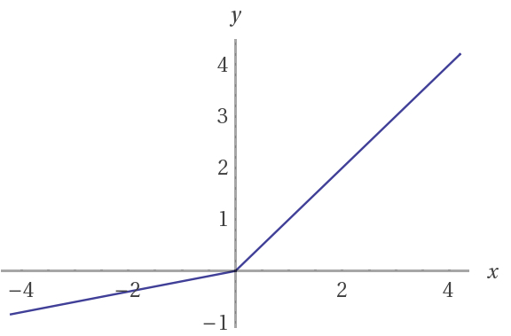
Activation functions: Relu

It has proved that 6 times improvement in convergence from Tanh function
Activation functions: Relu
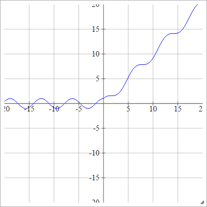
Activation functions: Gaussian
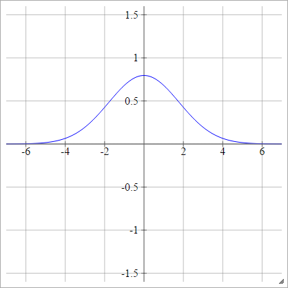
Activation functions:Multiquadratic
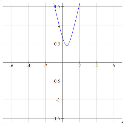
Activation functions:Softmax
Sigmoid function used for the two-class classification
Softmax function is used for the multi-class classification
Other Activation functions
- SWISH
- Cosine
- Maxout
- Inverse Multiquadratic
SIDE NOTEs about Activation functions
- Vanishing gradient problem
- Zero centered output
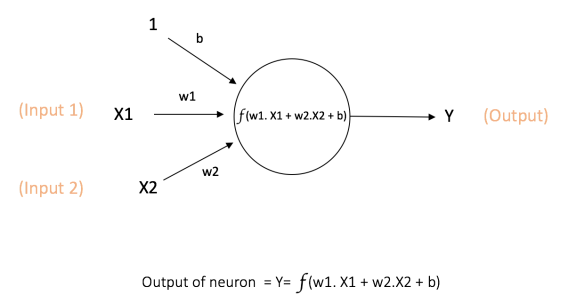
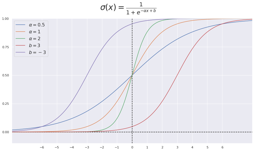
Bias
Bias allows us to shift the activation function to the left/right
Bias
Let's see some Examples
- Activation function:
NOT GATE
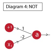

- Activation function:
OR GATE
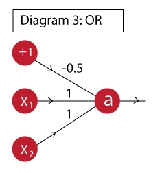

- Activation function:
And GATE
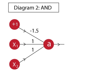

- Activation function:
A' . B' GATE
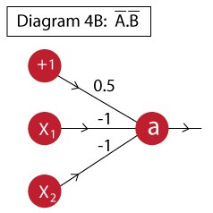

XNOR GATE
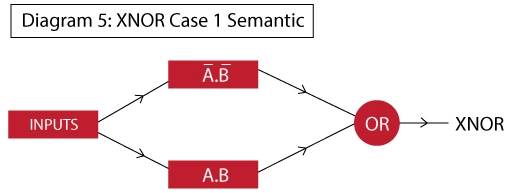
XNOR GATE
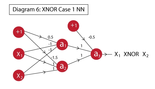

Network architecture is not unique!
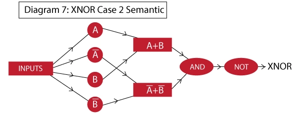
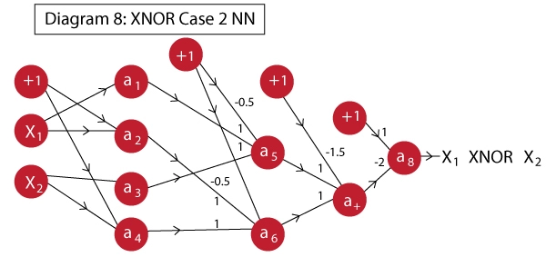
Seams easy, Nah?
Oh wait!
How can we find the weights?!
Can we implement XOR gate in a single neuron?
Before answer to this question let's ask a few more!
whats best architecture for our data?
Decision boundary
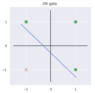
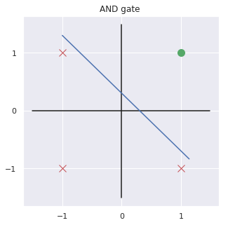
Decision boundary
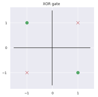
Regression vs single neuron
- Linear regression
- Single neuron
Regression vs single neuron
- Logistic regression
- Single neuron
Logistic Regression vs single neuron
A neural network is made up of multiple logistic regressions
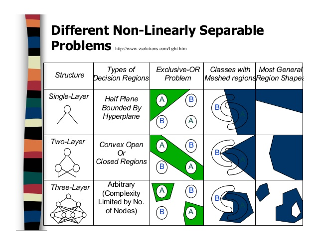
Summary
- Artificial Neural Networks are NON Linear classifiers
- Output of a single neuron is weighted sum affined by a non linear function
- More neurons means more complex decision boundries
BACKPROPAGATION Algorithm
unfortunately it's time to
DIVE INTO MATHEMATICS


In this section we focus on Supervised Learning to train our neural network
General Structure
We split our network to 3 main layers
- Input layer
- Hidden layers
- Output layer

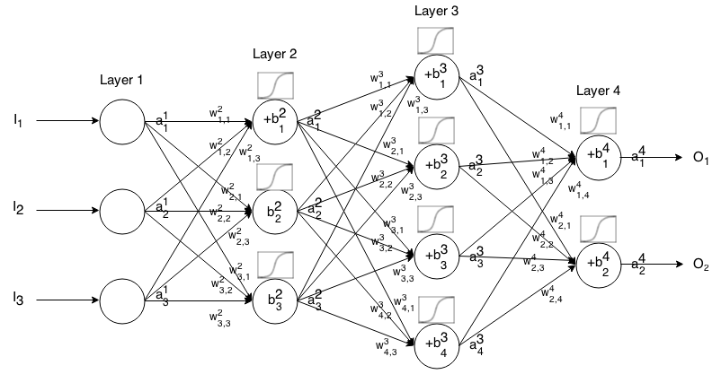
General Structure
This type of Artificial neural network known as MultiLayer Perceptron (MLP)
Since there is no cycle in this architecture we call this Feed Forward Network
Now can you guess why we shouldn't use linear activation function?
Lets start with an example
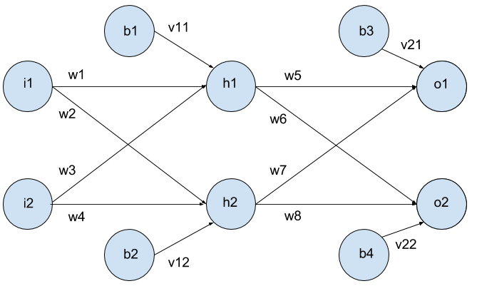
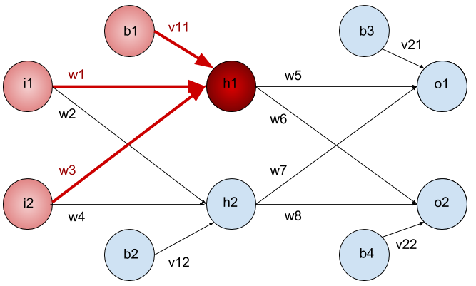

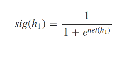
Whats \(net(h_2)\) and \(sig(h_2)\) ?
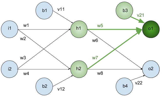

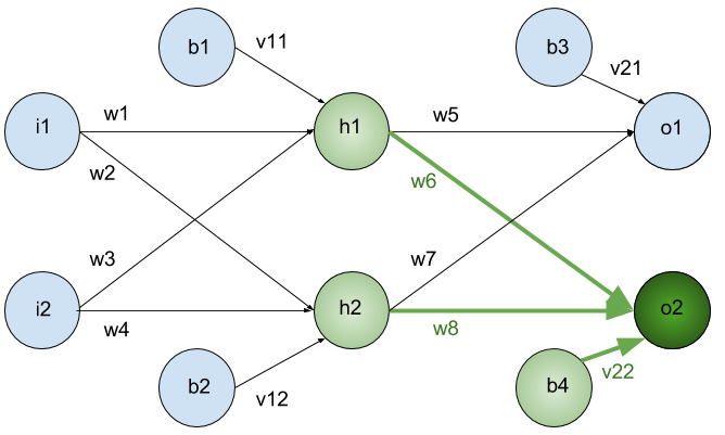


since we have target value of our samples (supervised learning) we can find the error of network predict as follow:
some times this called loss function
Where n = number of neurons at output layer

In our example:
In order to get best predicts we need to minimize error value
To minimize error we can:
- change bias
- change weights
- change previous activations!

since
As you saw this lost function has a quadratic form
It's obvious that this function may has much many variables
so we cant use calculus to find the minimum!
Learning algorithms
- Gradient descent
- Adam
- BFGS
- RMSProp
- . . .
- Newton's method
- Conjugate gradient
Learning algorithms
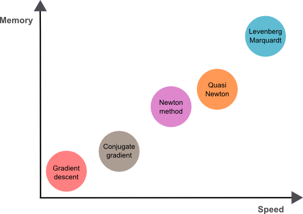
Here we focus on Gradient descent algorithm
Let's forget neural network aspects of this function
Just think you have a n-variable quadratic function and we want to minimize it
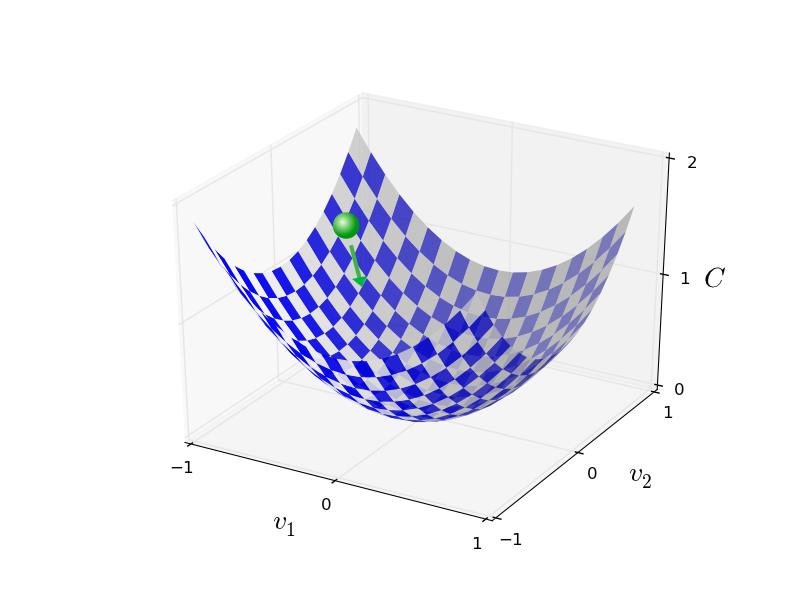
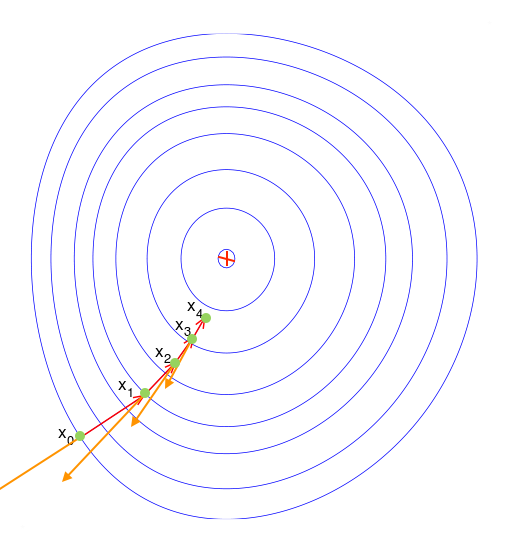
we simulate the random ball's rolling down motion by computing derivatives of function
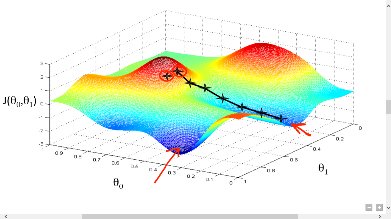

- Calculate slope at current position
- Updates parameters in opposite direction of gradient
Since
we are going to find a way to make \(\Delta C\) negative
Define:
So:
we want to make \(\Delta C\) negative since we look for a good \(\Delta v\)
let's suppose \(\Delta v = -\eta \nabla C^T\)
we had \(\Delta C \approx \nabla C \cdot \Delta v \) so:
Obviously \(\Delta C \lt 0\)
GOAL:
find \(\Delta v\) to change ball position in order to rich the functions minimum
if we do this over and over we rich global minimum
This approach works with more than two variable
gradient descent in neural network form
- Batch gradient descent
- Mini-Batch gradient descent
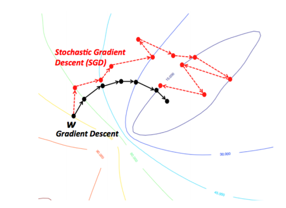
- Stochastic gradient descent
Gradient descent variants
Computes gradient with the entire dataset
- Pros:
- Guaranteed to converge to global/local minimum for convex/non-convex error surfaces
- Cons:
- Intractable for datasets that do not fit in memory
- Very slow
Batch gradient descent

Performs update for every mini-batch of n examples
- Pros
- Reduces variance of updates
- Can exploit matrix multiplication primitives
- Cons
- Mini-batch size is a hyperparameter
Mini-batch gradient descent
Same as Mini-batch but unit batch size on shuffled data
- Pros
- Much faster than batch gradient descent
- Allows online learning
- Cons
- High variance updates.
Stochastic gradient descent

BGD vs SGD
How to find \(\nabla C\)?
Backpropagation

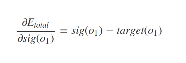


Derivative of sigmoid

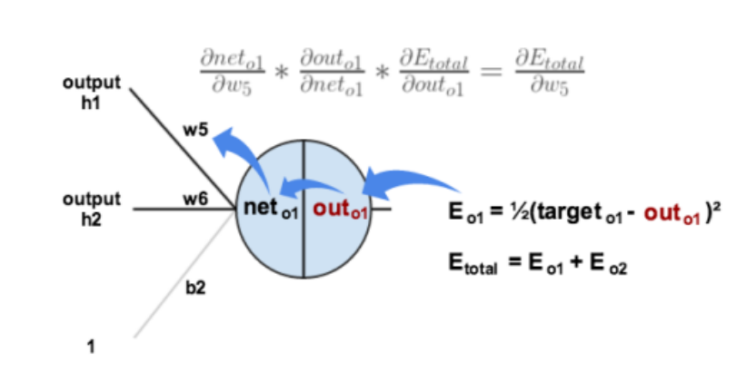


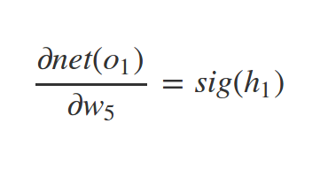

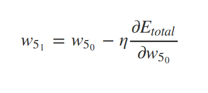
Similarly we have:


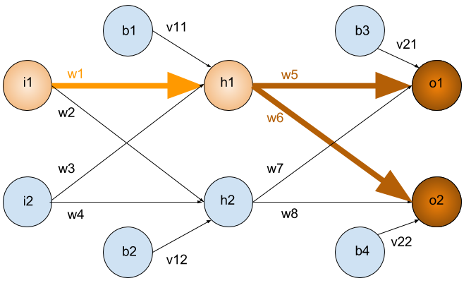
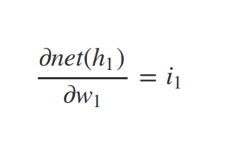
What about \(w_1\) ?


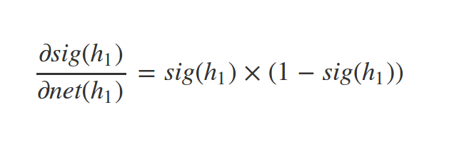
Similarly
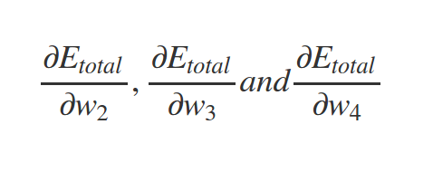
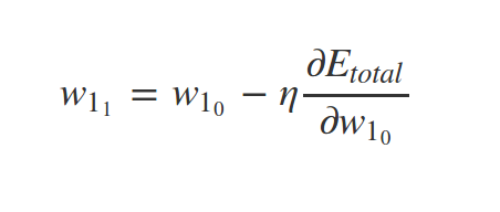
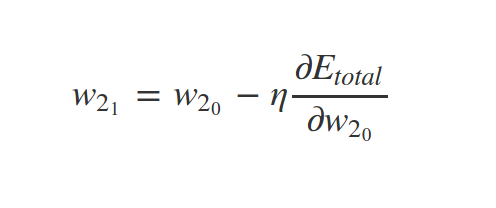
And so on . . .
What about biases?
Now you know why we need an activation function with big gradient for all inputs!
Why \(\eta\) ?

Local minimum and gradient descent!
http://iamtrask.github.io/2015/07/27/python-network-part2/

Summary
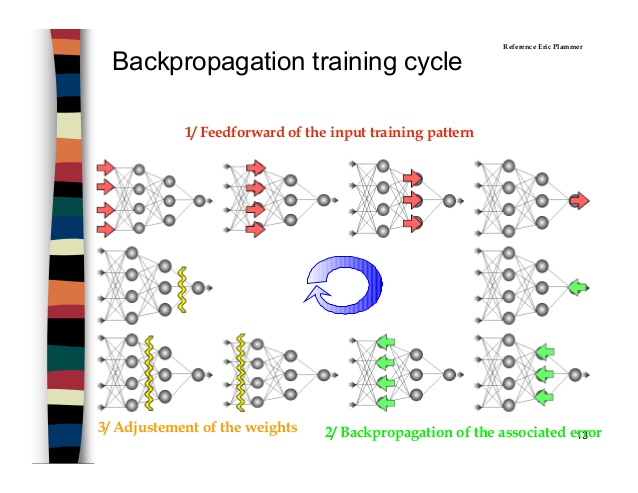
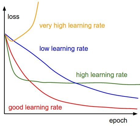
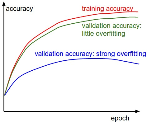
Data encoding
Categorical or Nominal data
Many machine learning algorithms cannot operate on label data
Data encoding
- Integer encoding
- Problem?
- One-hot encoding
- Binary encoding
- [More encodings]
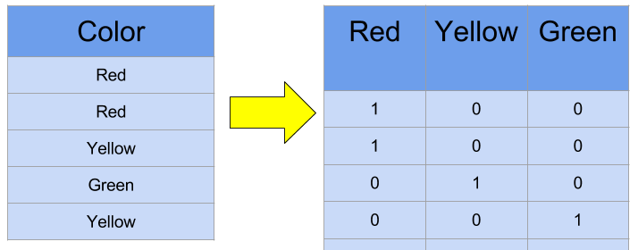
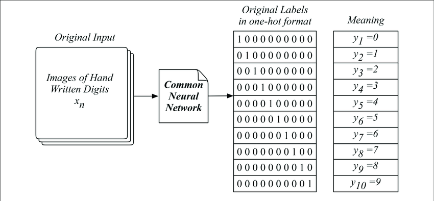
One-hot encoding
Softmax
Theorem.
2 layer MLP is a universal approximator
CNN
datasets: train,test,valid
over-fit, vs under-fit -> regulaization
fully connected-layer, dense
https://stats.stackexchange.com/questions/297749/how-meaningful-is-the-connection-between-mle-and-cross-entropy-in-deep-learning
https://stats.stackexchange.com/questions/167787/cross-entropy-cost-function-in-neural-network
https://datascience.stackexchange.com/questions/9302/the-cross-entropy-error-function-in-neural-networks
https://www.quora.com/What-are-the-differences-between-maximum-likelihood-and-cross-entropy-as-a-loss-function
https://aboveintelligent.com/deep-learning-basics-the-score-function-cross-entropy-d6cc20c9f972
https://en.wikipedia.org/wiki/Perceptron
delta rule,hebb,backpropagation,feed forward
https://medium.com/biffures/all-the-single-neurons-14de29a40f47
https://towardsdatascience.com/logistic-regression-detailed-overview-46c4da4303bc
https://en.wikipedia.org/wiki/Backpropagation
https://ml4a.github.io/ml4a/how_neural_networks_are_trained/
https://www.slideshare.net/MohdArafatShaikh/artificial-neural-network-80825958
https://juxt.pro/blog/posts/neural-maths.html
http://www.robertsdionne.com/bouncingball/
softmax probability vs sigmoid

References
- Fausett, L.V. and Fausett, L., Fundamentals of Neural Networks: Architectures, Algorithms, and Applications, 1994
-
KIYOSHI KAWAGUCHI, BSEE , A MULTITHREADED SOFTWARE MODEL FOR BACKPROPAGATION NEURAL NETWORK APPLICATIONS, 2000
- en.wikipedia.org/wiki/Neuron
- slideshare.net/neurosciust/what-is-a-neuron
- slideshare.net/HumaShafique/neuron-structure-and-function
- www2.fiit.stuba.sk/~kvasnicka/Seminar_of_AI/Benuskova_synplast.pdf
- slideshare.net/MohdArafatShaikh/artificial-neural-network-80825958
- https://towardsdatascience.com/activation-functions-and-its-types-which-is-better-a9a5310cc8f
- https://datascience.stackexchange.com/questions/26475/why-is-relu-used-as-an-activation-function
- https://medium.com/data-science-bootcamp/understand-the-softmax-function-in-minutes-f3a59641e86d
- http://www.themenyouwanttobe.com/data-science-resources/
- https://towardsdatascience.com/difference-between-batch-gradient-descent-and-stochastic-gradient-descent-1187f1291aa1
