Table of contents
- Introduction
- What is Tensorflow
- TF for Neural Networks
- Regression
- Classification
- TF for Function Approximation
- TF for Ordinary Differential Equations
- Keras for model definition
- DeepXDE
Introduction
Basics
- A high-performance numerical computation library.
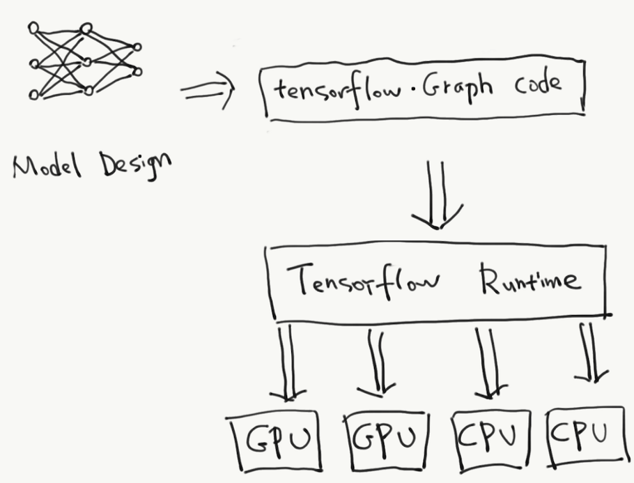
- Tensorflow supports
- Multidimensional-array based numeric computation
- CPU/GPU/TPU and distributed processing
- Automatic differentiation
- Model construction, training, and export
Basics
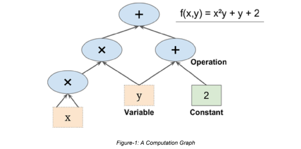
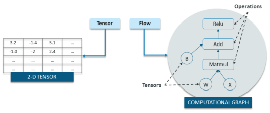
- In TensorFlow, computations are represented as computational graphs.
- Graphs are data structures that contain a set of operation objects, and tensor objects
- Operators represent units of computation
- Tensors represent the units of data that flow between operations.
Basics
Tensorflow
For Regression
A simple example
- Goal: Regression
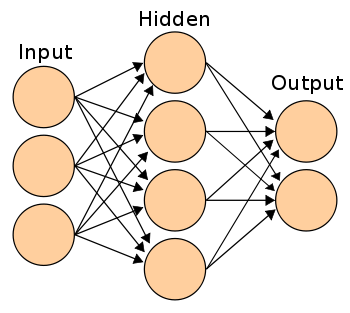
- Model: Multi-Layer Perceptron
- Dataset: Boston Housing
-
Samples: 506
-
Dimensionality: 13
-
Features: real, positive
-
A simple example
import tensorflow as tf

tf.random.set_seed(0)          # reproducible results

n_input = 13                   # number of features
n_hidden = 10                  # hidden layer size
n_output = 1                   # output layer size
w1 = tf.Variable(tf.random.normal([n_input, n_hidden]))
w2 = tf.Variable(tf.random.normal([n_hidden, n_output]))
b1 = tf.Variable(tf.random.normal([n_hidden]))
b2 = tf.Variable(tf.random.normal([n_output]))
optimizer = tf.optimizers.Adam()A simple example
def forward(x):
  hidden = x @ w1 + b1
  hidden = tf.nn.tanh(hidden)
  prediction = hidden @ w2 + b2
  return prediction
@tf.function
def step(X, y):
with tf.GradientTape() as tape:
prediction = forward(X)
loss = tf.losses.mean_squared_error(y_true=y, y_pred=prediction)
loss = tf.reduce_mean(loss)
weights = [w1, b1, w2, b2]
grads = tape.gradient(loss , weights)
optimizer.apply_gradients(zip(grads, weights))
return lossA simple example
from sklearn.datasets import load_boston

X, Y = load_boston(return_X_y = True)
X = X.astype('float32')
y = Y.reshape(-1,1)
losses = []
for i in range(5000):
loss = step(X, y)
losses.append(loss.numpy())import matplotlib.pyplot as plt
plt.plot(losses)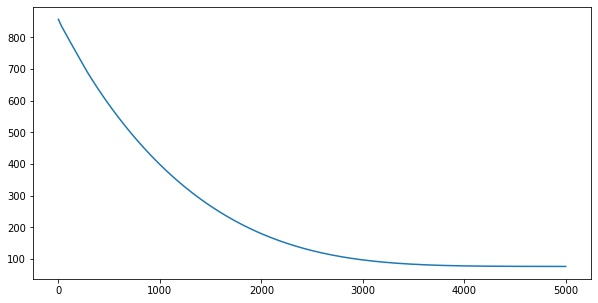
Tensorflow
For Classification
A simple example
- Goal: Binary Classification
- Model: Multi-Layer Perceptron
- Dataset: Breast Cancer
-
Samples: 569
-
Dimensionality: 30
-
Features: real, positive
-

A simple example
import tensorflow as tf

tf.random.set_seed(0)          # reproducible results

n_input = 30                   # number of features
n_hidden = 10                  # hidden layer size
n_output = 1                   # output layer size
w1 = tf.Variable(tf.random.normal([n_input, n_hidden]))
w2 = tf.Variable(tf.random.normal([n_hidden, n_output]))
b1 = tf.Variable(tf.random.normal([n_hidden]))
b2 = tf.Variable(tf.random.normal([n_output]))
optimizer = tf.optimizers.Adam()A simple example
def forward(x):
  hidden = x @ w1 + b1
  hidden = tf.nn.tanh(hidden)
  logits = hidden @ w2 + b2
  prediction = tf.nn.sigmoid(logits)
  return prediction
@tf.function
def step(X, y):
  with tf.GradientTape() as tape:
    prediction = forward(X)
    loss = tf.losses.binary_crossentropy(y_true=y, y_pred=prediction)
    loss = tf.reduce_mean(loss)

  weights = [w1, b1, w2, b2]
  grads = tape.gradient(loss , weights)
  optimizer.apply_gradients(zip(grads, weights))
  return loss
A simple example
from sklearn.datasets import load_breast_cancer

X, Y = load_breast_cancer(return_X_y = True)
X = X.astype('float32')
y = Y.reshape(-1,1)
losses = []
for i in range(2000):
loss = step(X, y)
losses.append(loss.numpy())import matplotlib.pyplot as plt
plt.plot(losses)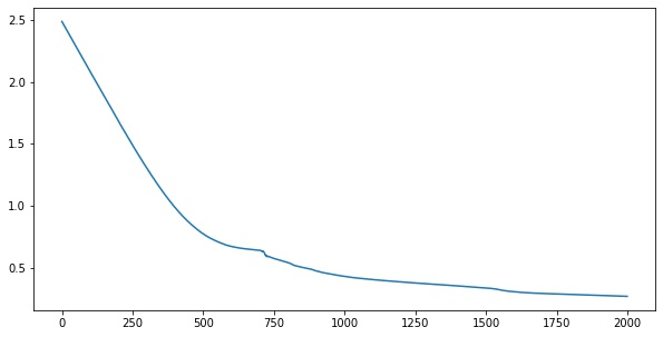
Tensorflow
For Function Approximation
A simple example
- Goal: Function Approximation
- Model: Multi-Layer Perceptron
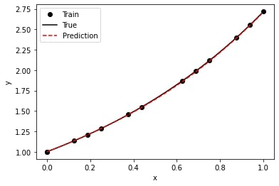
- Function: \(y(x)=e^x\)
- Domain: \(x=[0,1]\)

A simple example
import tensorflow as tf

tf.random.set_seed(0)          # reproducible results

n_input = 1                    # domain dimension
n_hidden = 5                   # hidden layer size
n_output = 1                   # range dimension
w1 = tf.Variable(tf.random.normal([n_input, n_hidden]))
w2 = tf.Variable(tf.random.normal([n_hidden, n_output]))
b1 = tf.Variable(tf.random.normal([n_hidden]))
b2 = tf.Variable(tf.random.normal([n_output]))
optimizer = tf.optimizers.Adam()A simple example
def forward(x):
  hidden = x @ w1 + b1
  hidden = tf.nn.tanh(hidden)
  prediction = hidden @ w2 + b2
  return prediction
@tf.function
def step(X, y):
with tf.GradientTape() as tape:
prediction = forward(X)
loss = tf.losses.mean_squared_error(y_true=y, y_pred=prediction)
loss = tf.reduce_mean(loss)
weights = [w1, b1, w2, b2]
grads = tape.gradient(loss , weights)
optimizer.apply_gradients(zip(grads, weights))
return lossA simple example
x = tf.linspace(0.0, 1.0, 100)

X = tf.reshape(x, (-1, 1))

y = tf.exp(X)
losses = []
for i in range(500):
loss = step(X, y)
losses.append(loss.numpy())import matplotlib.pyplot as plt
plt.plot(losses)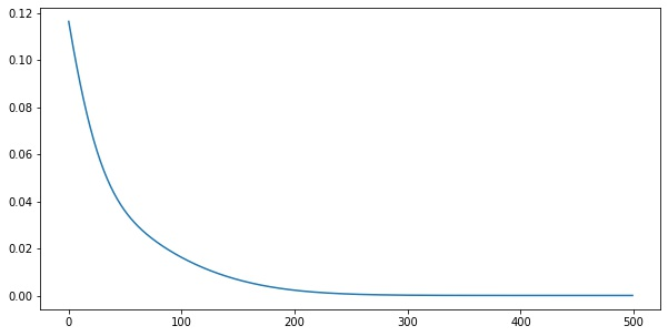
A simple example
import matplotlib.pyplot as plt
fig, axs = plt.subplots(1,2, figsize=(18,5))

domain = x.numpy()
exact = y.numpy().flatten()
predict = forward(X).numpy().flatten()

axs[0].plot(domain, exact, label='exact')
axs[0].plot(domain, predict, label='predict')
axs[0].legend()
axs[1].plot(domain, exact - predict, label='residual')
axs[1].legend()
Tensorflow
For Ordinary Differential Equations
A simple example
- Goal: Approximate the solution of
$$y'(x) = y(x)$$
- Model: Multi-Layer Perceptron
- Domain: \(x=[0,1]\)
- Exact Solution: \(y(x) = e^x\)

The Idea
- Approximate the solution of ODEs using a neural network.
- Approximated solution: \(\hat y(x)\)
- We already know:
$$\begin{aligned} y'(x) = y(x), \quad &\forall x\in [0,1]\Rightarrow \\ y'(x) - y(x) = 0, \quad &\forall x\in [0,1] \Rightarrow\\ y'(x_i) - y(x_i) = 0, \quad &x_i \in [0,1], i=1,2,\ldots,n. \end{aligned}$$
- What if \(\hat y(x)\) was not the exact solution?
The Idea
- Define the residual function as
$$Res(x; \hat y) = \hat y'(x) - \hat y(x)$$ - The residual function equals zero if and only if the approximated function \(\hat y\) is \(e^x\).
- Define the total error over all innerpoints, in a Mean Square Error (MSE) sense:
$$MSE = \frac{1}{n}\sum_{i=1}^n [Res(x_i; \hat y) - 0]^2$$
The Idea
- Is this methodology Supervised or Unsupervised?
- The target variable (Residual) must be Zero.
- The target variable is Zero for all inputs!
- \(MSE_{Res}\) can be interpreted as a complex loss function for a simple unsupervised network!
The Idea
- Do not forget the initial condition!
- Force the model to predict desired values.
$$Loss = \frac{1}{n}\sum_{i=1}^n Res(x_i; \hat y)^2 + [\hat y(0) - 1]^2$$
A simple example
import tensorflow as tf

tf.random.set_seed(0)          # reproducible results

n_input = 1                    # domain dimension
n_hidden = 10                  # hidden layer size
n_output = 1                   # range dimension
w1 = tf.Variable(tf.random.normal([n_input, n_hidden]))
w2 = tf.Variable(tf.random.normal([n_hidden, n_output]))
b1 = tf.Variable(tf.random.normal([n_hidden]))
b2 = tf.Variable(tf.random.normal([n_output]))
optimizer = tf.optimizers.Adam()A simple example
def forward(x):
  hidden = x @ w1 + b1
  hidden = tf.nn.tanh(hidden)
  y = hidden @ w2 + b2
  return y
@tf.function
def step(x):
weights = [w1, b1, w2, b2]
with tf.GradientTape() as tape:
y = forward(x)
dy_dx = tf.gradients(y, x)[0]
residual = dy_dx - y
boundary = y[0] - 1
loss = residual**2 + boundary**2
loss = tf.reduce_mean(loss)
grads = tape.gradient(loss, weights)
optimizer.apply_gradients(zip(grads, weights))
return lossA simple example
x = tf.linspace(0.0, 1.0, 100)
X = tf.reshape(x, (-1, 1))
losses = []
for i in range(100):
  loss = step(X, y)
  losses.append(loss.numpy())
import matplotlib.pyplot as plt
plt.plot(losses)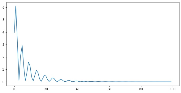
A simple example
import matplotlib.pyplot as plt
fig, axs = plt.subplots(1,2, figsize=(18,5))

domain = x.numpy()
exact = tf.exp(domain).numpy()
predict = forward(X).numpy().flatten()

axs[0].plot(domain, exact, label='exact')
axs[0].plot(domain, predict, label='predict')
axs[0].legend()

axs[1].plot(domain, exact - predict, label='residual')
axs[1].legend()

- Most used deep learning framework among top-5 winning teams on Kaggle.
- An industry-strength framework that can scale to large clusters of GPUs or an entire TPU pod.
- Take advantage of the full deployment capabilities of the TensorFlow platform.
- Keras is used by CERN, NASA, NIH, and many more scientific organizations around the world.
Basics
model = tf.keras.models.Sequential()
model.add(tf.keras.layers.Dense(10,input_shape=(1,),activation='tanh'))
model.add(tf.keras.layers.Dense(1, activation='linear'))
A simple example
Replace the weight/bias definitions and the forward function, with a sequential model!
@tf.function
def step(X, y):
  with tf.GradientTape() as tape:
    prediction = model(X)
    loss = tf.losses.mean_squared_error(y_true=y, y_pred=prediction)
    loss = tf.reduce_mean(loss)

  weights = model.trainable_weights
  grads = tape.gradient(loss , weights)
  optimizer.apply_gradients(zip(grads, weights))
  return loss
A simple example
- Call the sequential model, instead of forward function
- Use trainable weights for obtaining model weights
DeepXDE
For Ordinary/Partial Differential Equations
- A library for scientific machine learning, especially physics-informed learning algorithms, including:
- Physics-informed neural networks
- Deep operator networks
- Multifidelity neural networks
- Install it by:
Basics
pip install deepxdeA Simple Example
Import the required modules
Define the residual function
import deepxde as dde
import numpy as np
def residual(x, y):
y = y[:, 0:1]
dy_x = dde.grad.jacobian(y, x, i=0)
return [dy_x - y]A Simple Example
The boundary conditions
Define the exact solution for verification
def boundary(_, on_initial):
    return on_initial

geom = dde.geometry.TimeDomain(0, 1)
ic = dde.icbc.IC(geom, lambda x: 1, boundary)
def exact(x):
return np.hstack((np.exp(x), ))A Simple Example
Define the PDE system:
Define the neural network (function approximator)
data = dde.data.PDE(geom, residual, [ic],
                    num_boundary=2, solution=exact,
                    num_domain=10, num_test=100)
layer_size = [1] + [10] + [1]
activation = "tanh"
initializer = "Glorot uniform"
net = dde.nn.FNN(layer_size, activation, initializer)A Simple Example
Finally, connect the PDE system to the neural network
model = dde.Model(data, net)
model.compile("adam", lr=0.1, metrics=["l2 relative error"])
losshistory, train_state = model.train(epochs=1000)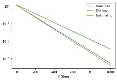
A Simple Example
