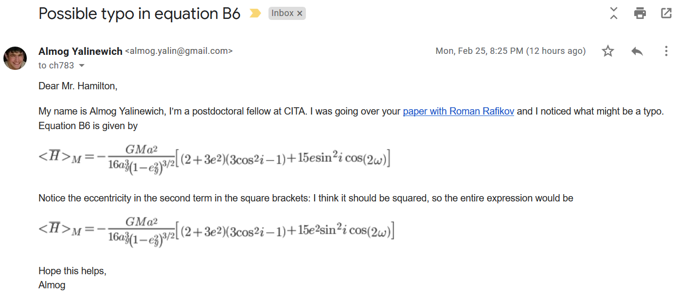
secular evolution of binaries in clusters

Secular dynamics of binaries in stellar clusters I: general

formulation and dependence on cluster potentia

Almog Yalinewich

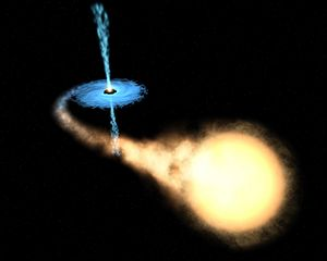
X ray binaries

a < 1 \, \rm AU

100x more common in clusters than in the field

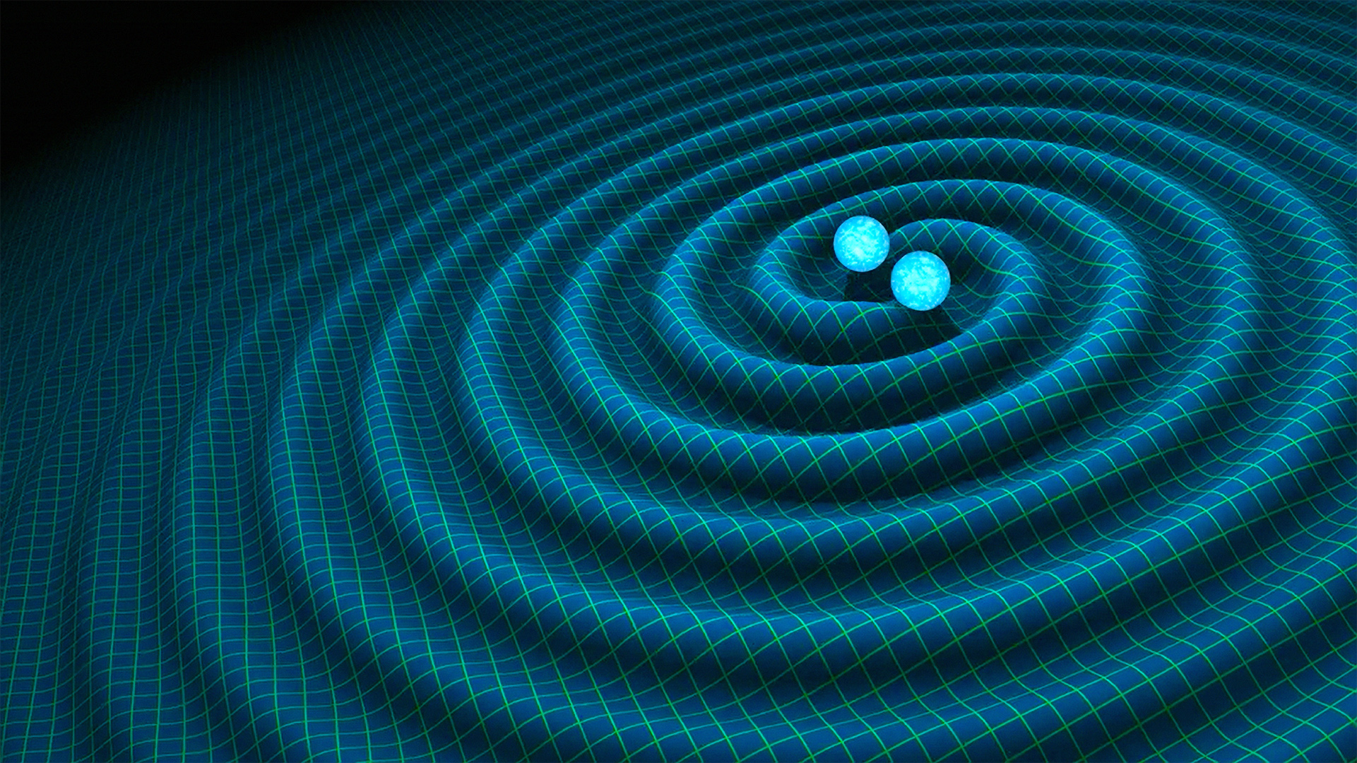
Gravitational waves

a < 3 \, \rm R_{\odot}

To merge within a Hubble time

Progenitors could not have formed that close

Gravitational waves - derivation

L \approx \frac{G}{c^5} \left(\frac{d^3 Q}{d t^3}\right)^2 \approx \frac{G}{c^5} \left(M a^2 \omega^3\right)^2

\omega^2 = \frac{G M}{a^3}

L \tau_H > \frac{G M^2}{a} \Rightarrow a < \left(\frac{G M}{c^2}\right)^{3/4} \left(c \tau_H\right)^{1/4}

Schwartzschild radius

size of the universe

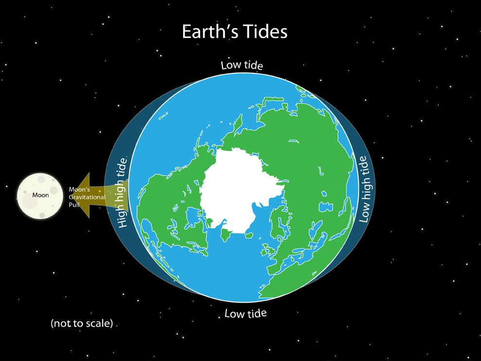
Binary in a Cluster

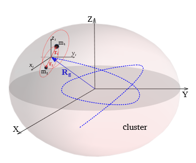
Tidal Field

\Phi \left(\vec{r}\right) \approx \Phi_0 + \vec{F} \cdot \Delta \vec{r}+ \Delta \vec{r} \cdot \overleftrightarrow{T} \cdot \Delta \vec{r}

gauge

centre of mass motion

Secular approximation

Binary period << Barycentre period

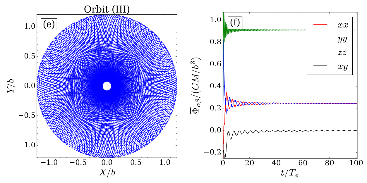
Orbits -> hoops

Hoop Energy

\Delta U = \int_V \vec{r} \overleftrightarrow{T} \rho \vec{r} d^3r= Tr \left[ \overleftrightarrow{T} \cdot \int_V \vec{r} \otimes \vec{r} \rho d^3 r \right]

Inertia tensor

\overleftrightarrow{I} = \int_V \vec{r} \otimes \vec{r} \rho d^3 r

For Keplerian Binary Orbits

\overleftrightarrow{I} = \frac{m}{T} \int_{0}^{T} \vec{r} \otimes \vec{r} dt

Keplerian Inertia Tensor

\textcolor{yellow}{r = \frac{r_l}{1+ e \cos \theta}}, \textcolor{cyan}{\dot{\theta} = \frac{l}{r^2}}

\frac{1}{m} \overleftrightarrow{I} = \frac{1}{T} \int_{0}^{T} \vec{r} \otimes \vec{r} \textcolor{red}{dt} = \frac{1}{T} \int_{0}^{\textcolor{red}{2 \pi}} \vec{r} \otimes \vec{r} \textcolor{red}{\frac{d \theta}{\dot{\theta}}} =

= \frac{1}{T \textcolor{cyan}{l}} \int_{0}^{2 \pi} \vec{r} \otimes \vec{r} \textcolor{cyan}{r^2} d \theta = \frac{\textcolor{yellow}{r_l^4}}{T l} \int_0^{2 \pi} \frac{\hat{r} \otimes \hat{r}}{\textcolor{yellow}{\left(1+e \cos \theta\right)^4}} d \theta

Solution of the Integral

\frac{T l}{r_l^4} \frac{I_{xx}}{m} = \int_0^{2 \pi} \frac{\cos^2 \theta d \theta}{\left(1+e \cos \theta\right)^4} = \frac{\pi \left(1+4 e^2\right)}{\left(1-e^2\right)^{7/2}}

I_{zz} = I_{zx} = I_{zy} = I_{xy} = 0

\frac{T l}{r_l^4} \frac{I_{yy}}{m} = \int_0^{2 \pi} \frac{\sin^2 \theta d \theta}{\left(1+e \cos \theta\right)^4} = \frac{\pi }{\left(1-e^2\right)^{5/2}}

Second Averaging

Keplerian Orbit

Almost any other potential

1D curve

2D surface

Convergence

Convergence 2

Convergence 3

Integration Variable

dt = \frac{dr}{v_r}

U = \Phi + \frac{1}{2} v_r^2 + \frac{1}{2} v_{\theta}^2 = \Phi + \frac{1}{2} v_r^2 + \frac{l^2}{r^2}

v_r = \sqrt{2\left(U-\Phi \right)-l^2/r^2 }

Integration Limits

U = \frac{r_a \Phi \left(r_a\right)-r_p^2 \Phi \left(r_a\right)}{r_a^2-r_p^2}

l = \sqrt{\frac{2 \left(\Phi \left(r_a\right) - \Phi \left(r_p\right)\right)}{r_p^{-2}-r_a^{-2}}}

\bar{F}=\frac{\int_{r_p}^{r_a} dr F \left(r \right)/v_r}{\int^{r_a}_{r_p} dr / v_r}

Cylindrical Coordinates

T_{xx} = T_{yy} = \frac{1}{2} \left[\frac{\partial^2 \Phi}{\partial r^2} + \frac{1}{r} \frac{\partial \Phi}{\partial r} \right]

T_{zz} = \frac{\partial^2 \Phi}{\partial z^2}|_{z=0}

T_{xy} = T_{xz} = T_{yz} = 0

Secular Hamiltonian

H = Tr\left[\overleftrightarrow{R}^T \overleftrightarrow{T} \overleftrightarrow{R} \overleftrightarrow{I} \right]

Axisymmetry

H \propto \left(2 + 3 e^2\right) \left(1- 3 \Gamma \cos^2 i\right) - 15 \Gamma e^2 \sin^2 i \cos 2 \omega

\Gamma= \frac{1}{3} \frac{T_{zz}-T_{xx}}{T_{zz}+T_{xx}}

Spherical Symmetry

H \propto 2+3 e^2

Kozai Lidov Mechanism

Keplerian potential

\Phi \propto \frac{1}{\sqrt{r^2+z^2}}

T_{zz} = -2 T_{xx} \propto \frac{1}{r^3}

\Gamma = 1

H \propto \left(2 + 3 e^2\right) \left(1- 3 \cos^2 i\right) - 15 e^2 \sin^2 i \cos 2 \omega

Heisler & Tremaine 1986

Vertical motion more important than horizontal

T_{xx} = 0

\Gamma = \frac{1}{3}

H \propto \left(2 + 3 e^2\right) \left(1- \cos^2 i\right) - 5 e^2 \sin^2 i \cos 2 \omega

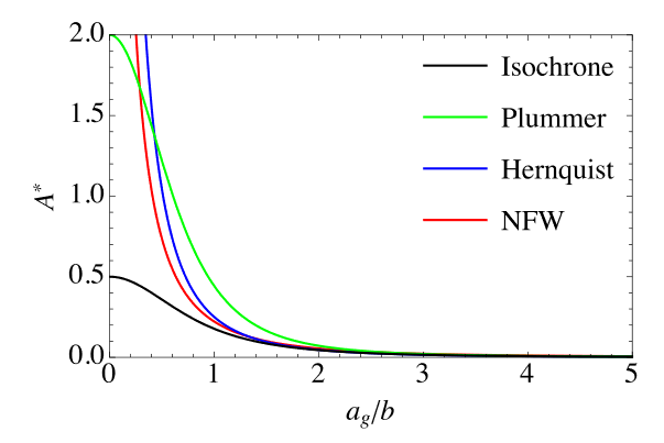
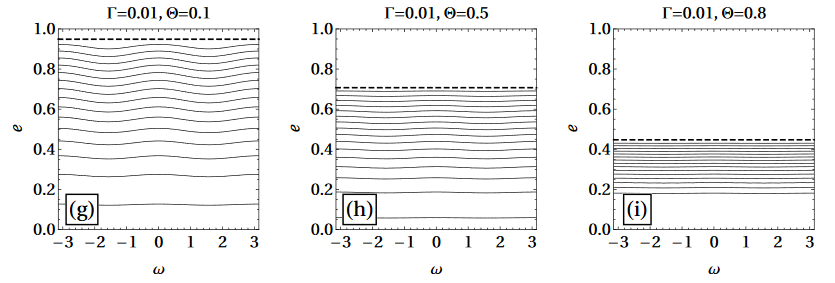
Anisotropy Parameter

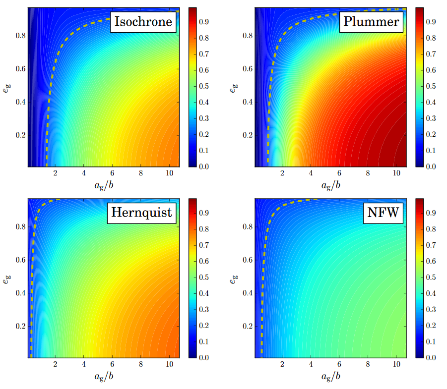
weak dependence on eccentricity

Anisotropy Parameter

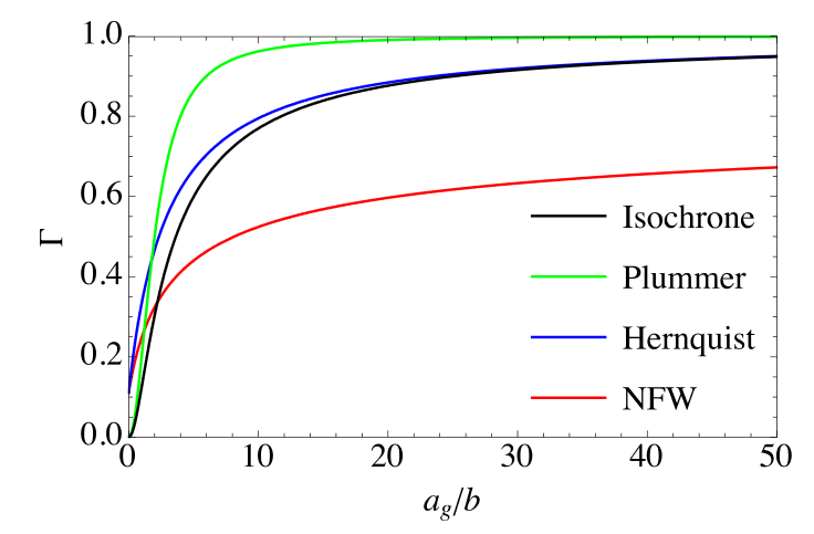
Coupling Constant

H = A f \left(e,i,\omega\right)

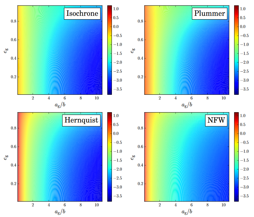
Almost indepedent of eccentricity

Coupling Constant

H = A f \left(e,i,\omega\right)

Dimensionless Hamiltonian

j = \sqrt{1-e^2}

\Theta = \left(1-e^2\right) \cos^2 i

H_1^* = \frac{1}{j^2} \left(j^2-3 \Gamma \Theta\right) \left(5-3j^2\right) - 15 \frac{\Gamma}{j^2} \left(j^2 -\Theta \right) \left(1-j^2\right) \cos 2 \omega

Integral of the motion

Time Evolution

Hamilton's Equations

\frac{d \omega}{d t} \propto \frac{\partial H^*_1}{\partial j} =

= \frac{6}{j^3} \left[5 \Gamma \Theta - j^4 +5 \Gamma \left(j^4 -\Theta\right) \cos 2 \omega\right]

\frac{d j}{d t} \propto -\frac{\partial H_1^*}{\partial \omega} = - \frac{30 \Gamma}{j^2} \left(j^2 -\Theta\right) \left(1-j^2 \right) \sin 2 \omega

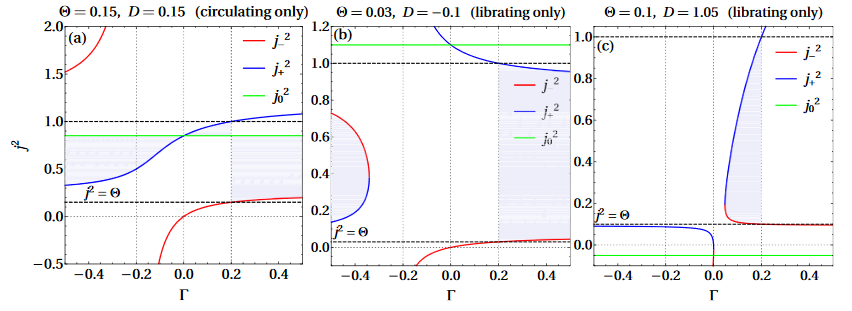
Non Trivival Fixed Points

\omega_f = \frac{\pi}{2}, j_f = \left(\frac{10 \Gamma \Theta}{1 + 5 \Gamma}\right)^{1/4}

\sqrt{\Theta} < j < 1

\Theta < \min \left(\frac{10 \Gamma}{1+5 \Gamma}, \frac{1+5 \Gamma}{10 \Gamma}\right)

By definition

Condition for existance of fixed points

Libration vs Circulation

Can you reach the top?

Libration vs Circulation

Unstable fixed point @

\omega = 0

j^2 = \frac{5/3 - 2 \Gamma \Theta -5 \Gamma -H_1^*/3}{1- 5 \Gamma}

\Theta < j^2 < 1

Recalling that

Condition for circulation

0 < D< 1 - \left(1-e^2\right) \cos^2 i

D = e^2 \left[1+\frac{10 \Gamma}{1 - 5 \Gamma} \sin^2 i \sin^2 \omega \right]

Extremal Eccentricities

\omega = 0

j_0 = \sqrt{1-D}

occur at fixed points

\omega = \frac{\pi}{2}

j_{\pm} = \sqrt{\frac{\Sigma \pm \sqrt{\Sigma^2 -10 \Gamma \Theta \left(1 + 5 \Gamma\right)}}{1+5 \Gamma}}

\Sigma = \frac{1 + 5 \Gamma}{2} + 5 \Gamma \Theta + \frac{5 \Gamma-1}{2} D

Extremal Eccentricities

Timescale for Change in Eccentricity

\frac{d j^2}{d t} \propto \sqrt{\left(25 \Gamma^2 -1 \right) \left(j_0^2 - j^2\right) \left(j_+^2 - j^2 \right) \left(j^2 - j_{-}^2\right) }

Oscillation timescale

P_s = \int^{j_{\max}^2}_{j_{\min}^2} \frac{d j^2}{d j^2/dt}

Order of magnitude estimate

P_s = \frac{P_c^2}{P_b}

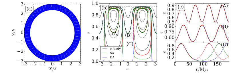
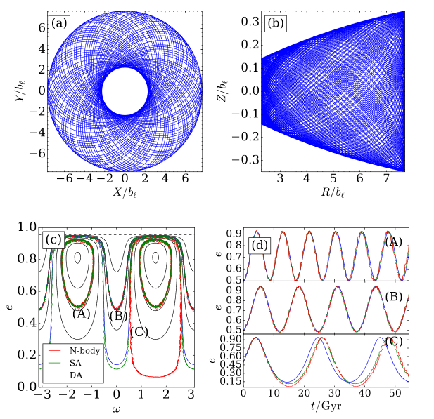
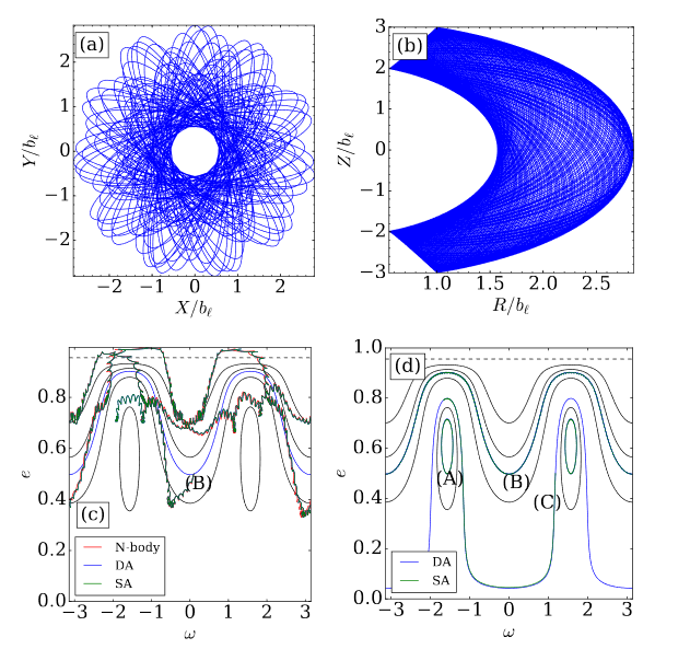
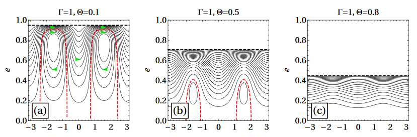
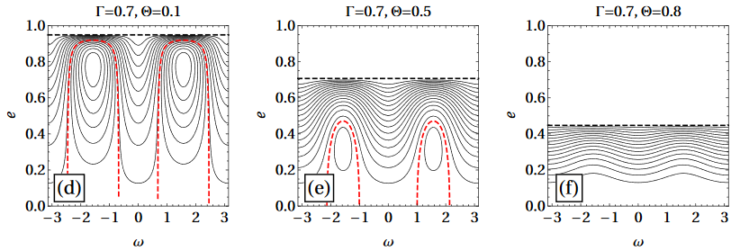
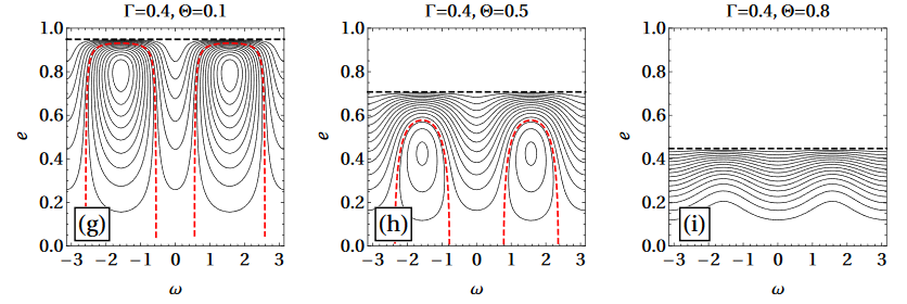
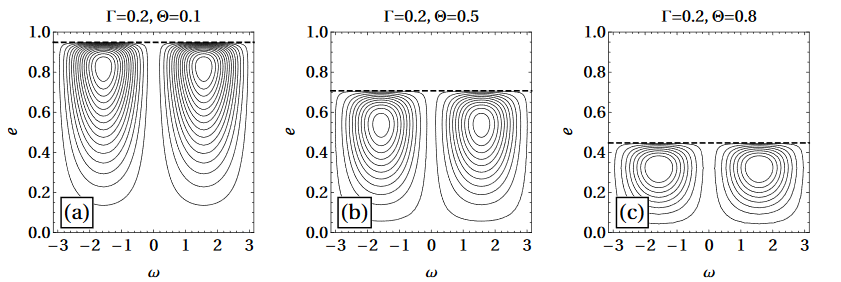
Phase Space Portraits

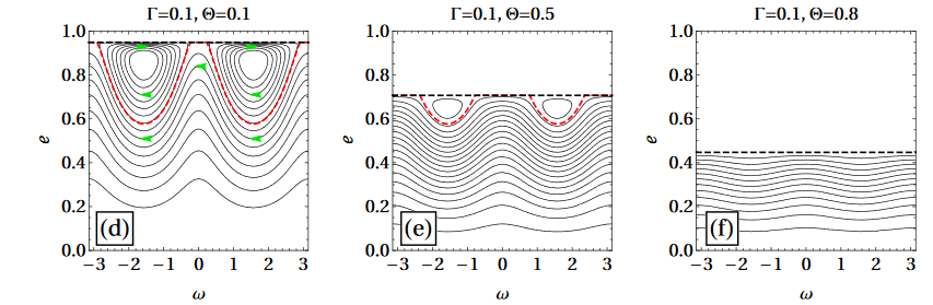
reversed separatrices for

\Gamma < \frac{1}{5}

Phase Space Portraits

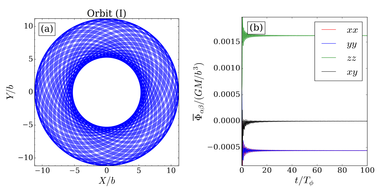
Verification

Isochrone Potential

\Phi = - \frac{G M}{b + \sqrt{b^2+r^2}}

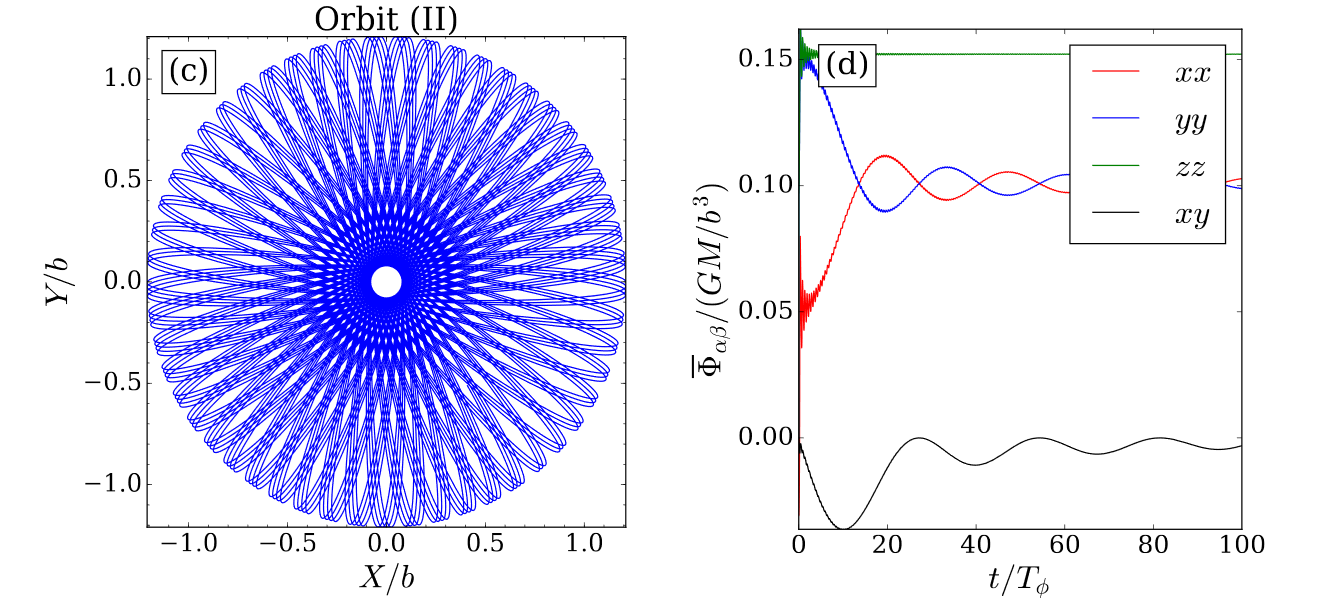
Verification

Miamoto Nagai Potential

\Phi = - \frac{G M}{\sqrt{R^2+\left(b_h+\sqrt{Z^2+b_h^2}\right)^2}}

time for neck stretches

Verification

Fit is not always that good for triaxial potentials

General Relativistic Potential

Paczynski Wiita potential

\Phi = \frac{G M}{r-R_g} \approx \frac{G M}{r} + \frac{G M R_g}{r^2}

Orbital Averaging

<\Delta \Phi> = - \frac{3 G^2 \left(m_1+m_2\right)^2}{c^2 a^2 \sqrt{1-e^2}}

\Delta \Phi

remains a constant

\Theta

Dimensionless Form

H_{GR}^* = - \frac{\varepsilon_{GR}}{j}

\varepsilon_{GR} \approx \frac{G^2 \left(m_1+m_2\right)^2}{c^2 a^2} / \frac{G M a^2}{b^3}

GR potential

tidal potential

Relativistic Precession

\dot{\omega}_{GR} = \frac{3 G^{3/2} \left(m_1+m_2\right)^{3/2}}{a^{5/2} c^2 \left(1-e^2\right)^{5/2}}

\frac{\dot{\omega}_{GR}}{\dot{\omega}_{NR}} \approx \frac{\varepsilon_{GR} j}{60 \Gamma \Theta}

Compared with tidal precession

Extremal Eccentricities

\Delta j_{\pm}^2 \approx \mp \frac{\varepsilon_{GR} j_{\pm}}{3 \left(1+5 \Gamma\right) \left(j_+^2-j_-^2\right)}

GR tends to make orbits less eccentric

\Delta j_0^2 \approx \frac{\varepsilon_{GR}}{3 \left(5 \Gamma-1\right)j_0}

Epilogue