KM-ε: A novel Categorical Clustering Algorithm

Mohamad Amin Mohamadi

Prof. Pasi Franti

Summer 2019

Cluster Analysis

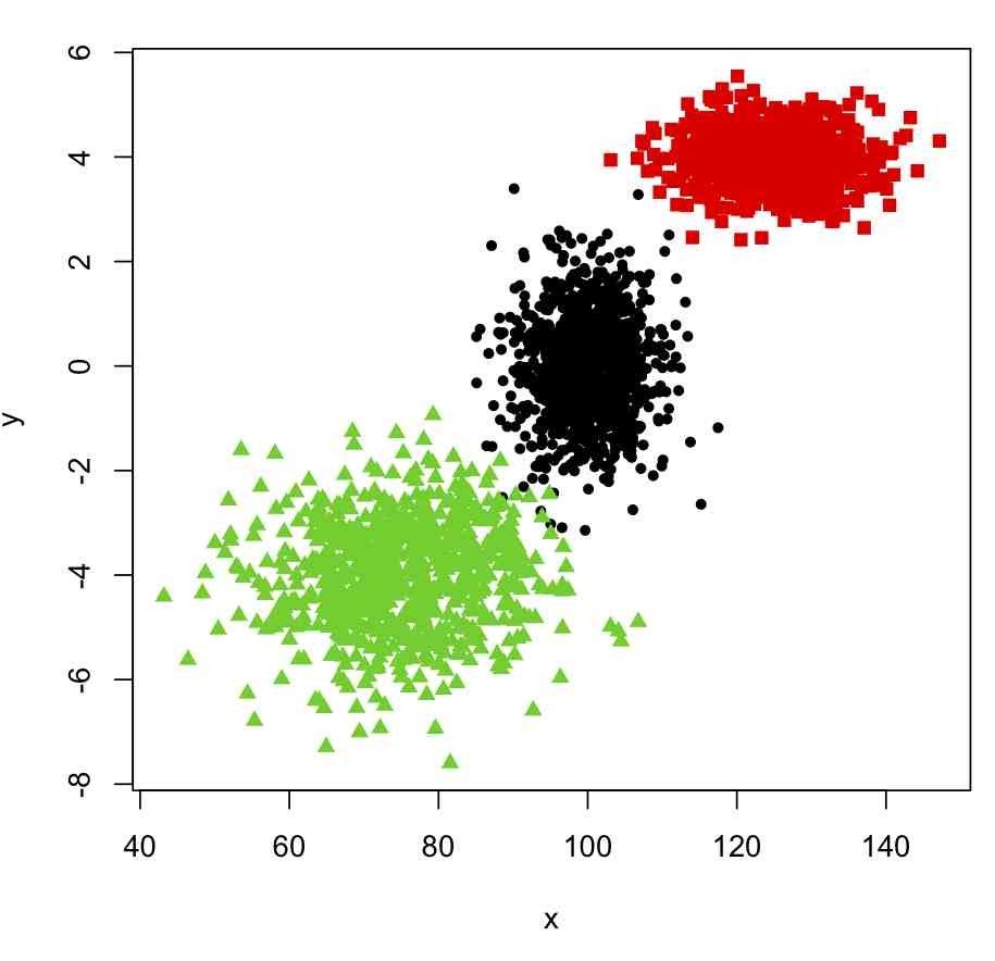
Categorical Data

Related Work

K-Means like iterative point of view
Agglomerative point of view
Direct optimization point of view
Subspace categorical clustering
Fuzzy categorical clustering

Motivation

Lack of optimal convergence guarantee and dependence of the solution to the initialization
High time complexity for optimal convergence (quadratic for special cases or more for general algorithms)
Need for extra convergence parameters
Need for pre or post processing of clustering results

Idea

Objective Function

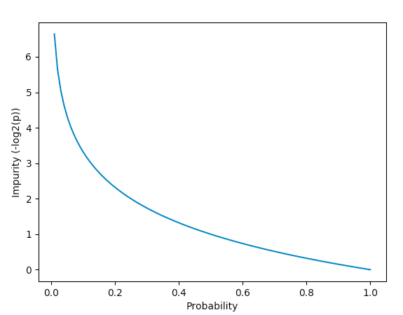
Using entropy as a measure of

purity in clusters

\sum_{j \in 1..k}{H(C_j) * (n_j / N)}

H(C_j): \text{Entropy of cluster } j \\ k: \text{Number of clusters} \\ n_j: \text{Size of cluster } j \\ N: \text{Number of data points} \\ X: \text{Input dataset with D attributes}

K-means Like Algorithm for Categorical Data

1. Centroid Step:

Calculate probabilities of each category in each attribute for clusters as for each cluster, where is the maximum number of categories in attributes.

2. Assignment step:

Assign each data point to the cluster where is:

j = \argmin -\sum_{a \in 1..D}{ln(C^{(j)}_{ax^a})} \qquad (1)

x = (x_1, x_2, ..., x_D)

C^{(j)} \in \mathbb{R}_{D \times C'}

C^{(j)} \text{ for } j \in 1..k

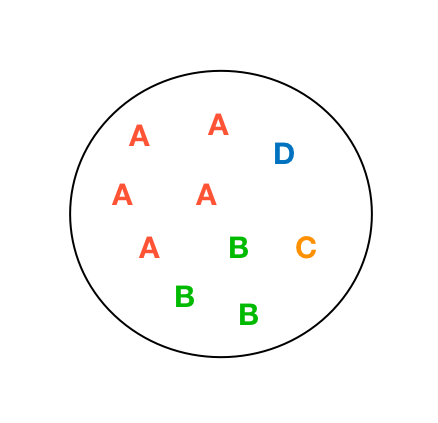
A Toy Example

N=10, D=4

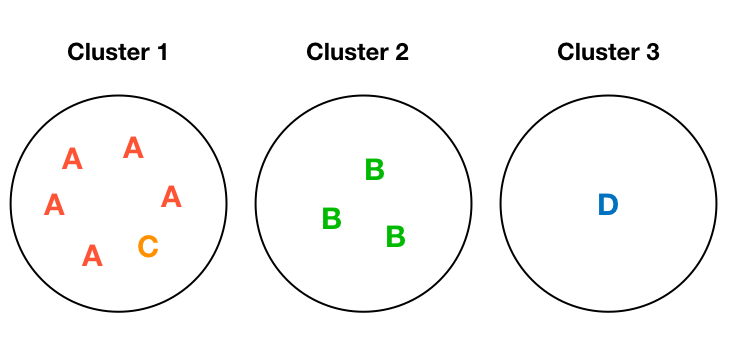
Entropy: 0

Entropy: 0.45

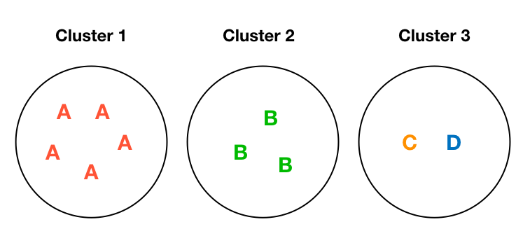
\text{Total entropy: } \frac{6}{10} \times 0.45 + \frac{3}{10} \times 0 + \frac{1}{10} \times 0 = 0.27

A Toy Example (Optimum)

N=10, D=4

Entropy: 0

Entropy: 0.69

Entropy: 0

\text{Total entropy: } \frac{5}{10} \times 0 + \frac{3}{10} \times 0 + \frac{2}{10} \times 0.69 = 0.14

Calculating Centroids

	P(A)	P(B)	P(C)	P(D)
Cluster 1	0.83	-	0.17	-
Cluster 2	-	1.00	-	-
Cluster 3	-	-	-	1.00

Assigning Datapoints

Cluster 1	Cluster 2	Cluster 3	Selected
0.18			1
	0		2
1.79			3
		0	1

x = A

x = B

x = C

x = D

\infty

We select the best cluster for each datapoint according to equation (1).

Assigning Datapoints

Problem:

Log of 0 is infinite, so the datapoints won't move if D-1 attributes feel comfortable about a move, but only one attribute doesn't!

Motivation:

Decrease the influence of categories with zero probability. Anticipate newcomers in less crowded clusters!

No datapoint moves! Each datapoint has it's best situation (according to eq. 1) in its own cluster!

Epsilon Strategy

\text{Cost} = \infty

* Costs Calculated according to equation 1

Epsilon Strategy

p = 0.0 \\ -log(p) = \infty

p = 0.1 (\epsilon) \\ -log(p) = 3.32

Calculating Centroids (Epsilon Strategy)

Let's start with a simple epsilon:

\epsilon = 1 / (n_j + 1) \\ p = p \times \frac{n_j}{n_j + 1}

Calculating Centroids (Epsilon Strategy)

	P(A)	P(B)	P(C)	P(D)
Cluster 1	0.67	0.17	0.17	0.17
Cluster 2	0.25	0.75	0.25	0.25
Cluster 3	0.5	0.5	0.5	0.5

Assigning Datapoints (Epsilon Strategy)

Cluster 1	Cluster 2	Cluster 3	Selected
0.40	1.38	0.69	1
1.77	0.28	0.69	2
1.77	1.38	0.69	3
1.77	1.38	0.69	3

We select the best cluster for each datapoint according to equation (1).

x = A

x = B

x = C

x = D

Assigning data points with epsilon idea

Datapoint C moves from cluster 1 to cluster 3
No other datapoints move afterwards
Reached the global optimum!

How To Choose Epsilon?

\epsilon = 1 / (n_j + 1)

\epsilon = 1 / N

Strategy	Average Impurity	Impurity SE
	7.59*	0.31*
	7.49*	0.26*

* Over 100 tests on the test dataset

Pseudo-Code: KM-ε

Input
-------------
X (N × D)
k
update_proportion_criterion

Algorithm
-------------
assign datapoints randomly to k clusters
do
    centroids = calculate_centroids()
    movements = assign_datapoints(centroids)
while movements > update_proportion_criterion * N

Pseudo-Code: KM-ε

function calculate_centroids()    
  for j in 1..k
    cluster_data = items in cluster j  // n_j * D matrix
    for d in 1..D
      if there is empty category in dimension d of cluster_data:
        for each category in dimension d as cat:
          if count(cat) in cluster_data > 0:
            centroids[k][d][cat] = count(cat) / (n_j + 1)
          else:
            centroids[k][d][cat] = 1 / (n_j + 1)
      else:
          for each category in dimension d as cat:
            centroids[k][d][cat] = count(cat) / n_j
  return centroids

Pseudo-Code: KM-ε

function assign_datapoints(centroids) 
  movements = 0
  for i in 1..N:
    selected_cluster = -1
    most_entropy = -infinite
  	for j in 1..k:
      cluster_entropy = 0
      for d in 1..D:
      	category = X[i][d]
        cluster_entropy -= log(centroids[j][d][category])
      if cluster_entropy > most_entropy:
        most_entropy = cluster_entropy
        selected_cluster = j
    if selected_cluster != prev_cluster[i]:
      movements++
      move datapoint to selected_cluster
  return movements

Testing The Algorithm

Mushroom dataset

For testing the algorithm, we used mushroom dataset.

Mushroom dataset properties:

8124 rows
22 attributes (all categorical)

We used 16 clusters for the mushroom dataset.

Results of running the algorithm on the dataset are available in the next slides.

Empirical results: KM-ε

Results of 100 runs:

Statistic	Value
Average impurity	7.49
Best (lowest) impurity	7.04
Worst (highest) impurity	8.12
Standard error of impurity	0.26
Empty cluster situations*	9

* By empty cluster situation, we mean that in some point the algorithm created some empty cluster and we couldn't continue the algorithm from there and thus, that case was dumped from the statistics

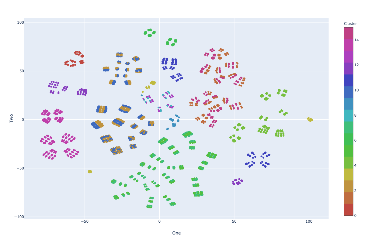
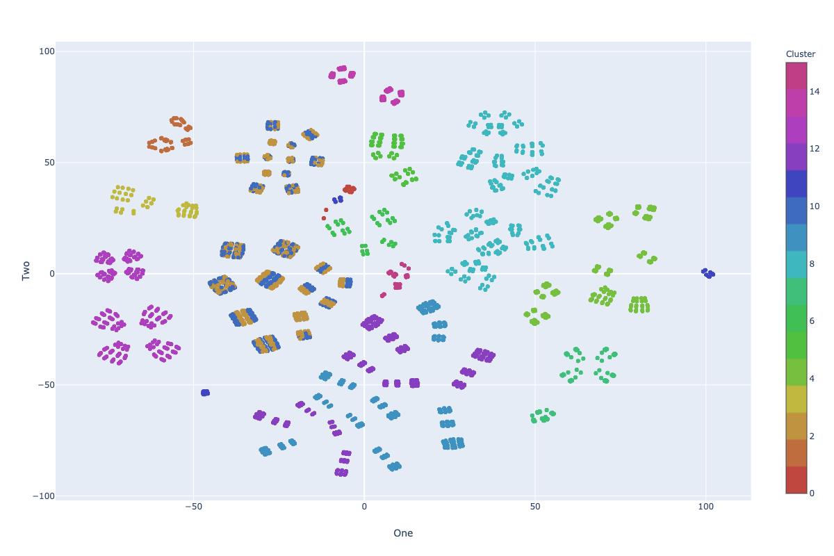
Visualization: KM-ε

Impurity: 7.41

* Visualization in 2D using TSNE

Far From Optimum

Improvement?

Add Random Swap

Random Swap

KM-ε + Random Swap

Result of 100 runs:

Statistic	Value
Average impurity	7.13
Best (lowest) impurity	6.98
Worst (highest) impurity	7.90
Standard error of impurity	0.13
Empty cluster situations*	4

* By empty cluster situation, we mean that in some point the algorithm created some empty cluster and we couldn't continue the algorithm from there and thus, that case was dumped from the statistics

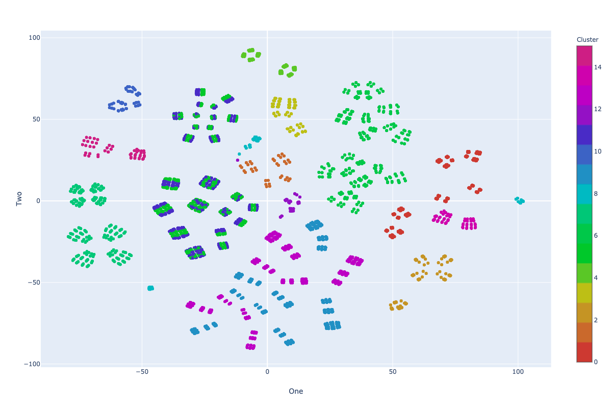
Visualization: KM-ε + Random Swap

Impurity: 7.10

Stress Test: KM-ε + Random Swap

For checking the rate of convergence of the algorithm, we tested the algorithm with 5000 random swaps to see if it achieves the overall impurity of <= 6.98 (reached with 100 random swap at least once) or not.
The result was NO!, the impurity achieved using 5000 random swaps was 6.99.

Other Assignment Strategies

The other assignment strategies tested were:
1. SE Strategy: Assigning the datapoints to the cluster with minimum distance where distance is defined as:
2. SE-Full Strategy: Assigning the datapoints to the cluster with minimum distance where distance is defined as

j = \argmin \sum_{a \in 1..D}{(1 - C^{(j)}_{ax_a})^2}

j = \argmin \sum_{a \in 1..D}{(1 - {C^{(j)}_{ax_a})}^2 + \sum_{a' \in 1..cats_a \wedge a' \ne x_a}{{C^{(j)}_{a'x_{a'}}}^2}}

* where cats represents the categories in an attribute

Results: SE Strategy

Here are the statistics of algorithm runs on mushroom dataset using the SE strategy assignment .

* By empty cluster situation, we mean that in some point the algorithm created some empty cluster and we couldn't continue the algorithm from there and thus, that case was dumped from the statistics

	K-Means (100 Runs)	K-Means + 100 Random Swaps (50 Runs)
Average impurity	7.51	6.99
Best (lowest) impurity	7.00	6.95 (New best)
Worst (highest) impurity	8.79	7.07
Standard error of impurity	0.13	0.02
Empty cluster situations*	27	2

Stress test visualization: SE Strategy

Impurity: 6.95

Stress test: SE Strategy

We reached the overall impurity of 6.95 during our tests with 100 random swaps in this strategy, which is a new best achieved clustering.
For checking the rate of convergence of the algorithm, we tested the algorithm with 10000 random swaps to see if it achieves the overall impurity of <= 6.95 (reached with 100 random swap at least once) or not.
The result was Yes!, the impurity achieved using 5000 random swaps was 6.95, which can indicate the stable convergence in SE strategy.

Strategy Comparison

Impurity	Epsilon = 1/N	SE Strategy
Average	7.013	6.99
Best (lowest)	6.98	6.95
Worst (highest)	7.90	7.07
Standard error	0.13	0.02

Strategy Comparison

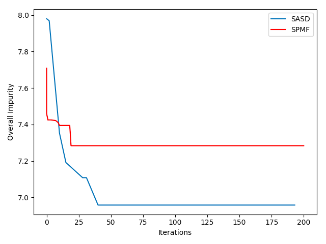
Convergence comparison plot for SE strategy (SASD) and initial epsilon 1/N

Strategy Comparison

According to the statistics achieved using the experiments, it seems like SE strategy has much faster convergence rate compared to the epsilon strategy, and this is probably because of the epsilon not being a good anticipation of the future changes in the next iterations of the algorithm. But in general, a good epsilon should give the best convergence rate.

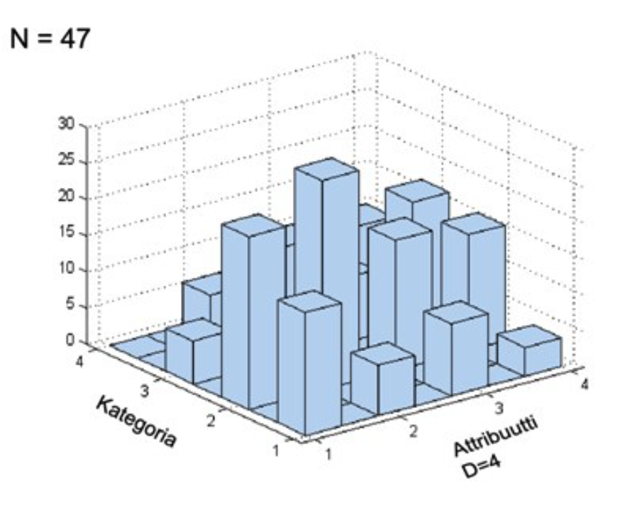
Internal Evaluation

Algorithm	Soybean M = 4 Cost std	Mushroom M = 16 Cost std	SPECT M = 8 Cost std
ACE	7.83 0	7.01 n/a	8.43 0.07
ROCK	9.20 0	n/a n/a	10.82 0
K-medoids	10.94 1.57	13.46 0.71	10.06 0.44
K-modes	8.66 1.06	10.19 1.45	9.25 0.29
K-distributions	9.00 0.93	7.87 0.44	8.25 0.13
K-represantives	8.30 0.83	7.51 0.30	8.64 0.13
K-histograms	8.04 0.53	7.31 0.18	8.64 0.15
K-entropy	8.15 0.56	7.31 0.18	8.06 0.07
Proposed	7.83 0	6.95 0	7.97 0

External Evaluations

To be added soon

Conclusion

Proposed new algorithm: KM-ε
- Optimal convergence guaranteed with adequate number of random swaps independent of the initialization
- Linear time complexity
- No extra convergence parameters
- No pre or post processing of clusters
Future Work
- Better anticipation of ε to have much higher rate of convergence
- Clustering mixed (numeric + categorical) data using the proposed concept

KM-ε: A novel Categorical Clustering Algorithm

Cluster Analysis

Categorical Data

Related Work

Motivation

Idea

Objective Function

Using entropy as a measure of

purity in clusters

K-means Like Algorithm for Categorical Data

A Toy Example

A Toy Example (Optimum)

Calculating Centroids

Assigning Datapoints

Assigning Datapoints

Epsilon Strategy

Epsilon Strategy

Calculating Centroids (Epsilon Strategy)

Calculating Centroids (Epsilon Strategy)

Assigning Datapoints (Epsilon Strategy)

Assigning data points with epsilon idea

How To Choose Epsilon?

Pseudo-Code: KM-ε

Pseudo-Code: KM-ε

Pseudo-Code: KM-ε

Testing The Algorithm

Mushroom dataset

Empirical results: KM-ε

Visualization: KM-ε

Far From Optimum

Improvement?

Add Random Swap

Random Swap

KM-ε + Random Swap

Visualization: KM-ε + Random Swap

Stress Test: KM-ε + Random Swap

Other Assignment Strategies

Results: SE Strategy

Stress test visualization: SE Strategy

Stress test: SE Strategy

Strategy Comparison

Strategy Comparison

Strategy Comparison

Internal Evaluation

External Evaluations

To be added soon

Conclusion

Proposed new algorithm: KM-ε