A tale of ∞-wide neural networks
Mohamad Amin Mohamadi
September 2022
Math of Information, Learning and Data (MILD)
Outline
- The Neural Tangent Kernel
- Training dynamics of ∞-wide neural networks
- Approximating the training dynamics of finite neural networks
- Linear-ized neural networks
- Applications of the Neural Tangent Kernel
(Our work included)
- Approximating the Neural Tangent Kernel
(Our work)
1. The NTK
Deep Neural Networks
- Over-parameterization often leads to fewer "bad" local minimas, albeit the non-convex loss surface
- Extremely large networks that can fit random labels paradoxically achieve good generalization error on test data (kernel methods ;-) ?)
- The training dynamics of deep neural networks is not yet characterized
Training Neural Networks
Basic elements in neural network training:
Gradient Descent:
Training Neural Networks
Idea: Study neural networks in the function space!
Gradient Flow:
Change in the function output:
Hmm, looks like we have a kernel on the right hand side!
Training Neural Networks
So:
where
this is called the Neural Tangent Kernel!
Training Neural Networks


Arthur Jacot, Franck Gabriel, Clement Hongler
∞-wide networks
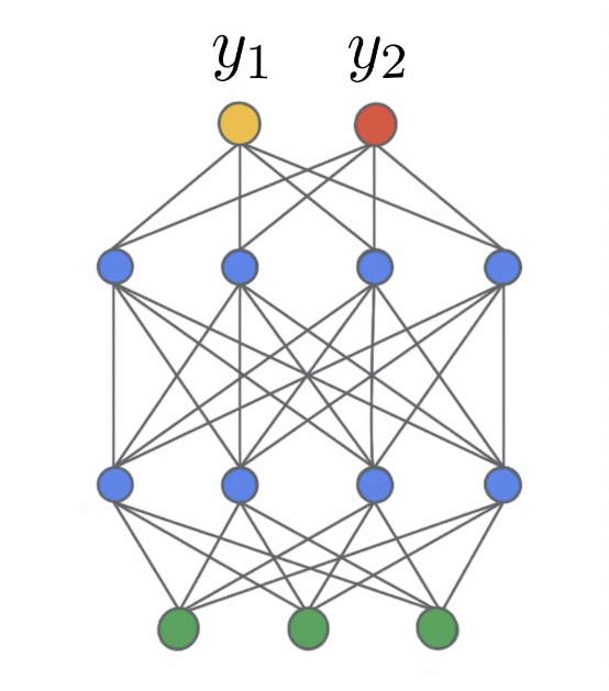
- (Theorem 1) For an MLP network with depth L at initialization, with a Lipschitz non-linearity, at the limit of infinitely wide layers, the NTK converges in probability to a deterministic limiting kernel.
∞-wide networks
- (Theorem 2) For an MLP network with depth with a Lipschitz twice-differentiable non-linearity, at the limit of infinitely wide layers, the NTK does not change during training along the negative gradient flow direction.
- Now, What does this imply?
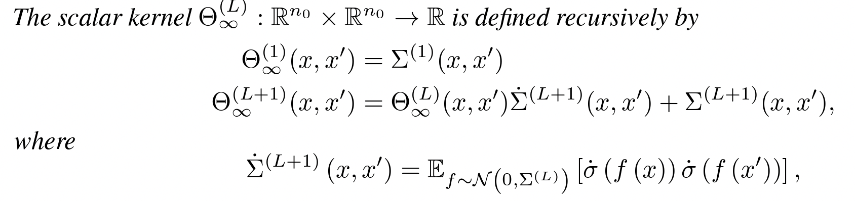
∞-wide networks
- If the kernel is constant in time, we can solve this system of differential equations! (Stack the training points)
- If the kernel is constant, we can claim global convergence based on the PSD-ness of the limiting kernel (Proven for a general case).
∞-wide networks
Thus, we can analytically characterize the behaviour of infinitely wide (and obviously, overparameterized) neural networks, using a simple kernel ridge regression formula!
As it can be seen in the formula, convergence is faster along the kernel principal components of the data (early stopping ;-) )
Finite wide networks
- As we saw, convergence and training dynamics of infinitely-wide neural networks can be captured using a simple kernel regression-alike formula (?)
- Does this have any implication for finite neural networks?
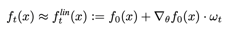
Finite wide networks
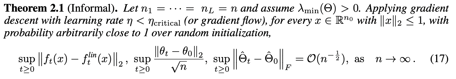
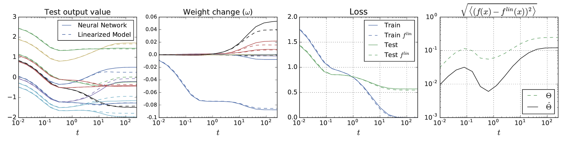
Lee et al. showed that the training dynamics of a linear-ized version of a neural network can be explained using kernel ridge regression with the kernel as the empirical Neural Tangent Kernel of the network:
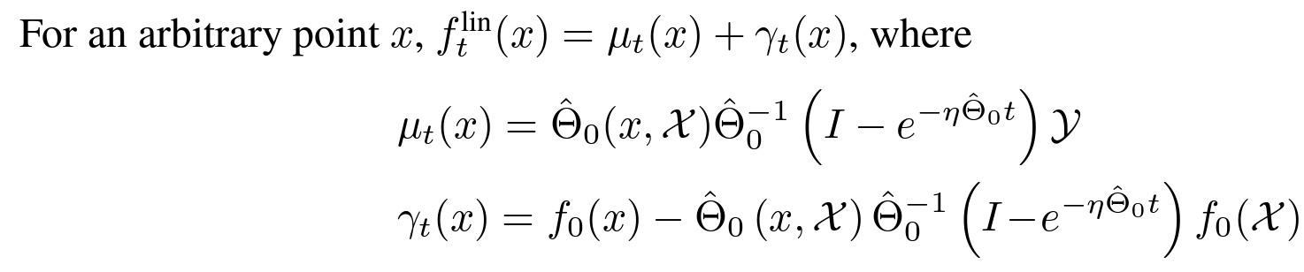
Finite wide networks
More importantly, they provided new approximation bounds for the predictions of the finite neural network and the linear-ized version:
2. Applications of the Neural Tangent Kernel
NTK Applications
-
NTK Has enabled lots of theoretical insights into deep NNs:
- Studying the geometry of the loss landscape of NNs (Fort et al. 2020)
- Prediction and analyses of the uncertainty of a NN’s predictions (He et al. 2020, Adlam et al. 2020)
-
NTK Has been impactful in diverse practical settings:
- Predicting the trainability and generalization capabilities of a NN (Xiao et al. 2018 and 2020)
- Neural Architecture Search (Park et a. 2020, Chen et al. 2021)
NTK Applications
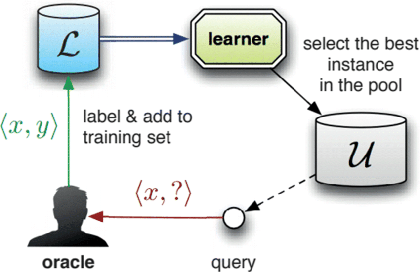
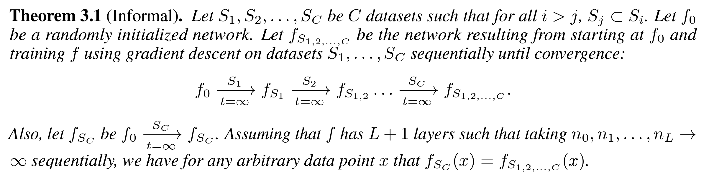
- We used NTK in pool-based active learning to enable "look-ahead" deep active learning
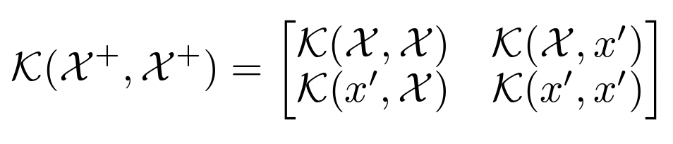
- Main idea: Approximate the behaviour of model after adding a new datapoint using a linear-ized version!
NTK Applications
NTK Applications
3. Approximating the Neural Tangent Kernel
NTK Computational Cost
-
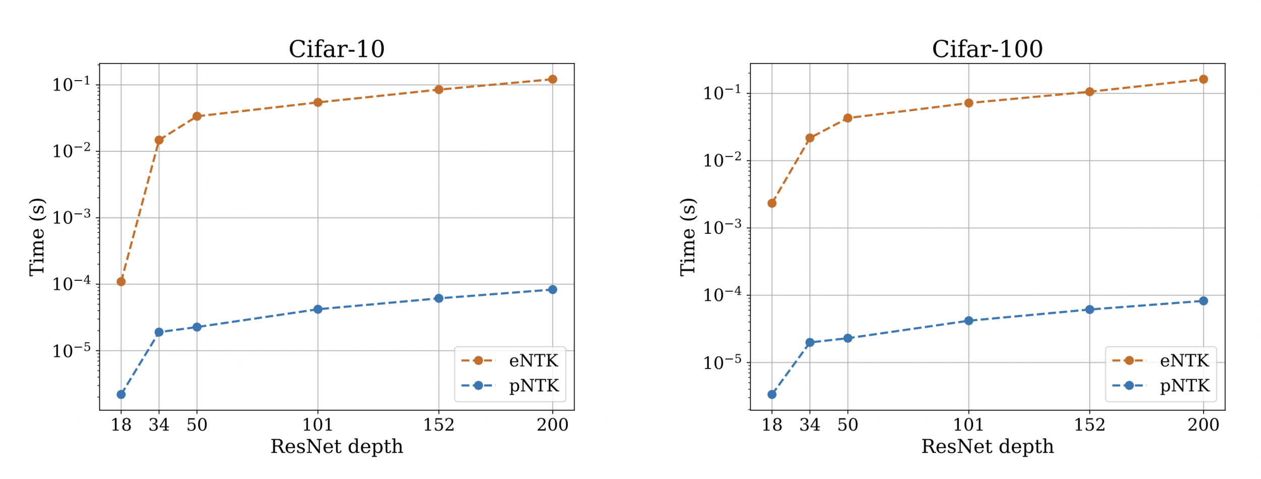
Is, however, notoriously expensive to compute :(
- Both in terms of computational complexity, and memory complexity!
- Computing the Full empirical NTK of ResNet18 on Cifar-10 requires over 1.8 terabytes of RAM !
-
Our recent work:
- An approximation to the NTK, dropping the O term from the above equations!
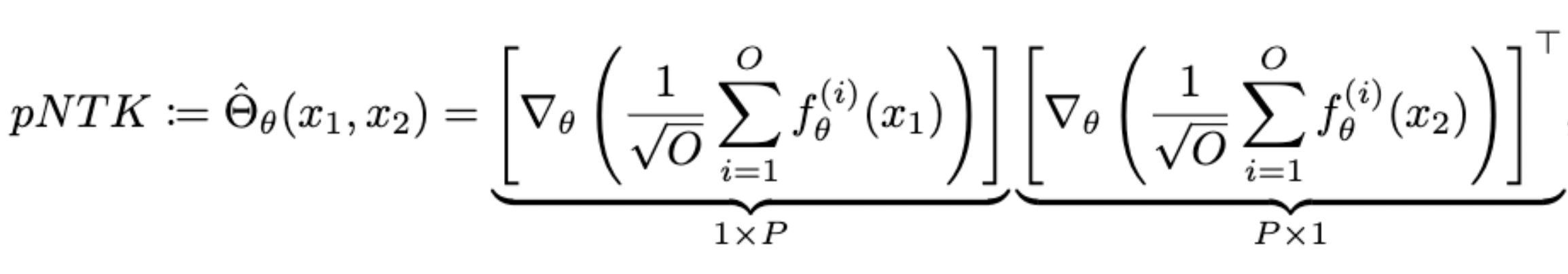
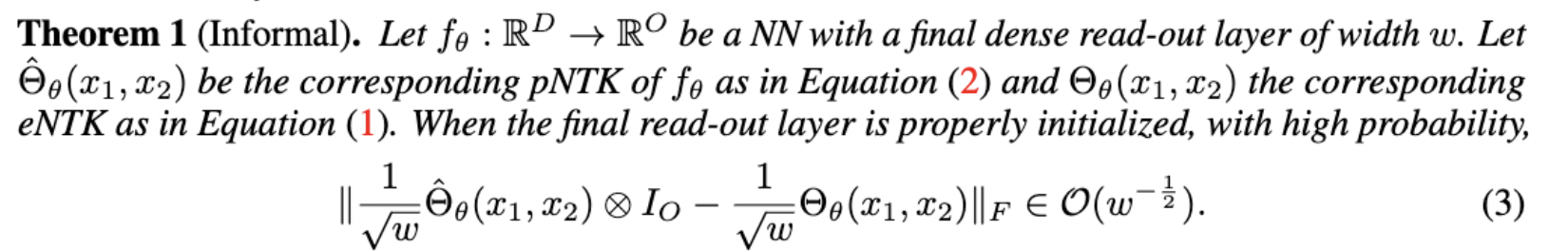
An Approximation to the NTK
- For each NN, we define pNTK as follows:
- Computing this approximation requires less time and memory complexity (Yay!)
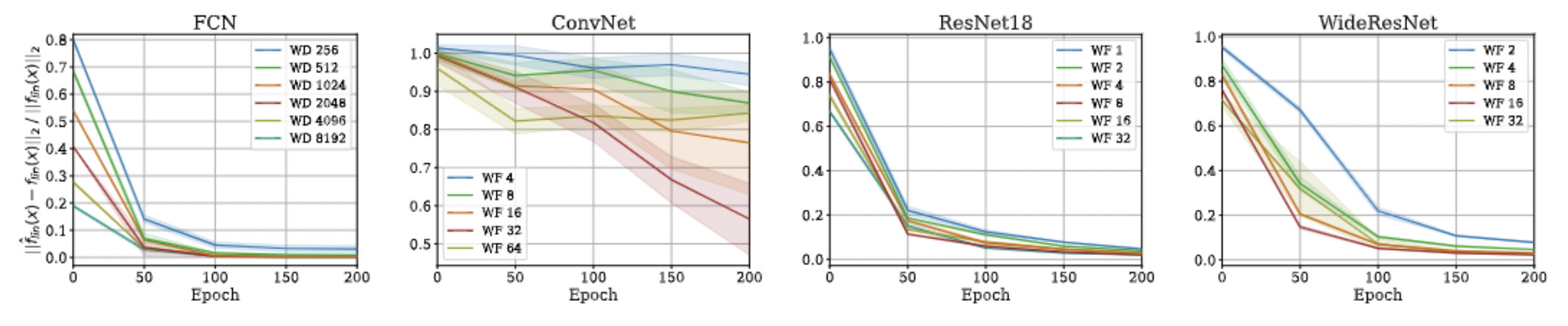
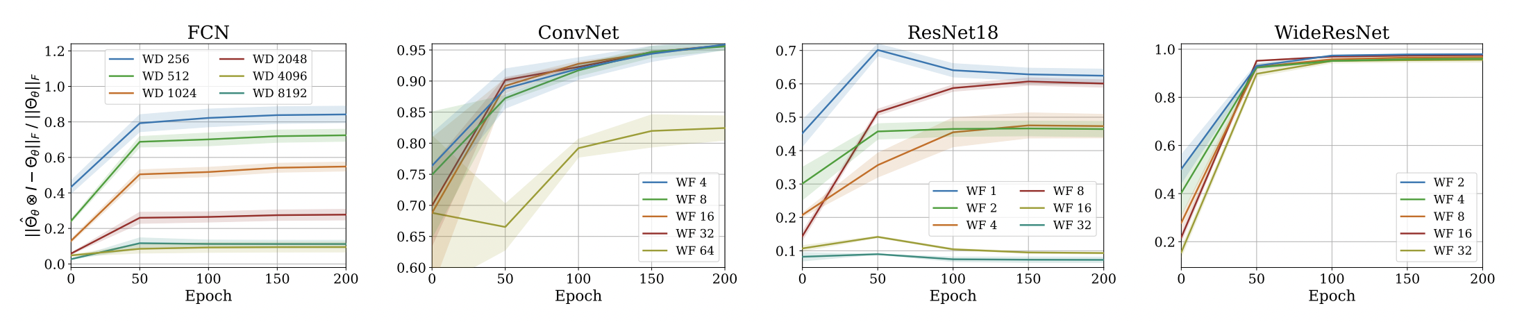
Approximation Quality: Frobenius Norm
- Why?
- The diagonal elements of the difference matrix grow linearly with width
- The non-diagonal elements are constant with high probability
- Frobenius Norm of the difference matrix relatively converges to zero
Approximation Quality: Frobenius Norm
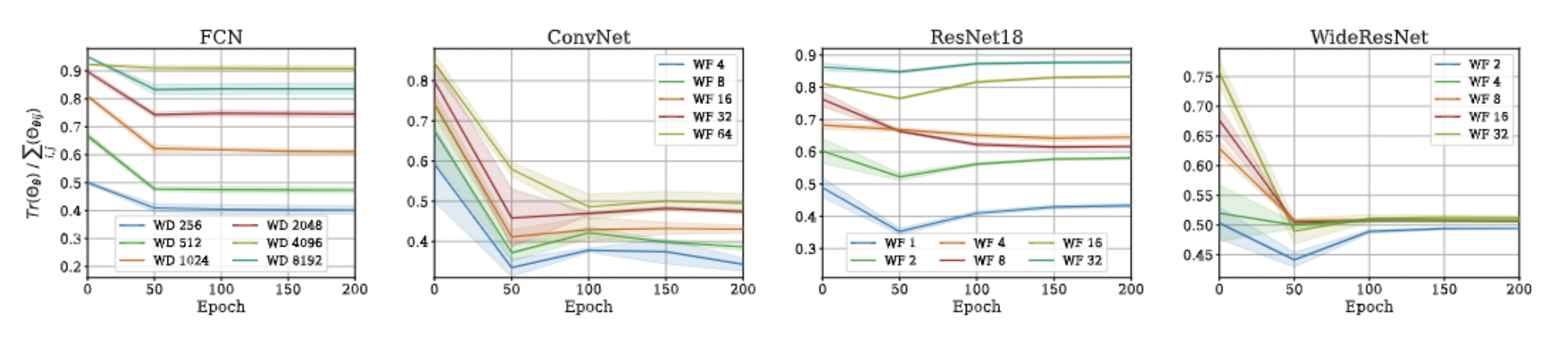
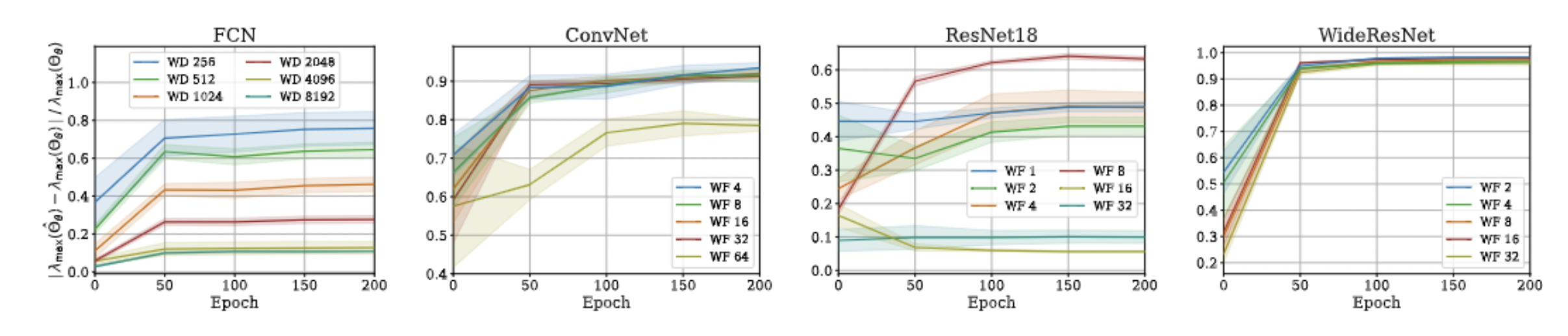
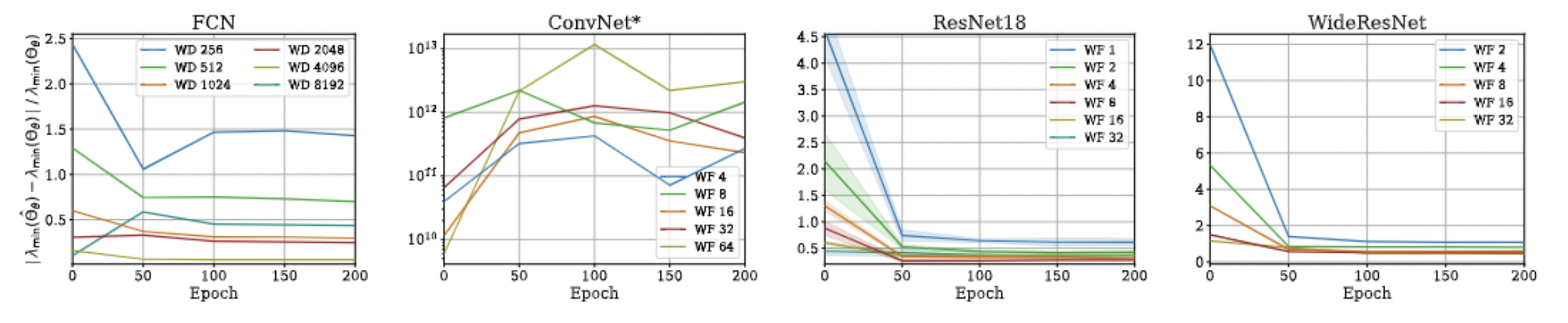
Approximation Quality: Eigen Spectrum
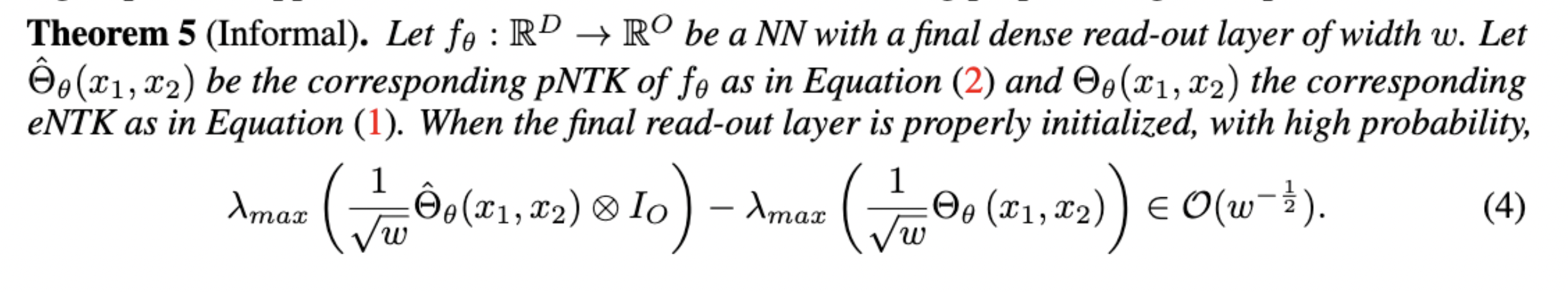
- Proof is very simple!
- Just a triangle inequality based on the previous result!
- Unfortunately, we could not come up with a similar bound for min eigenvalue and correspondingly the condition number, but empirical evaluations suggest that such a bound exists!
Approximation Quality: Eigen Spectrum
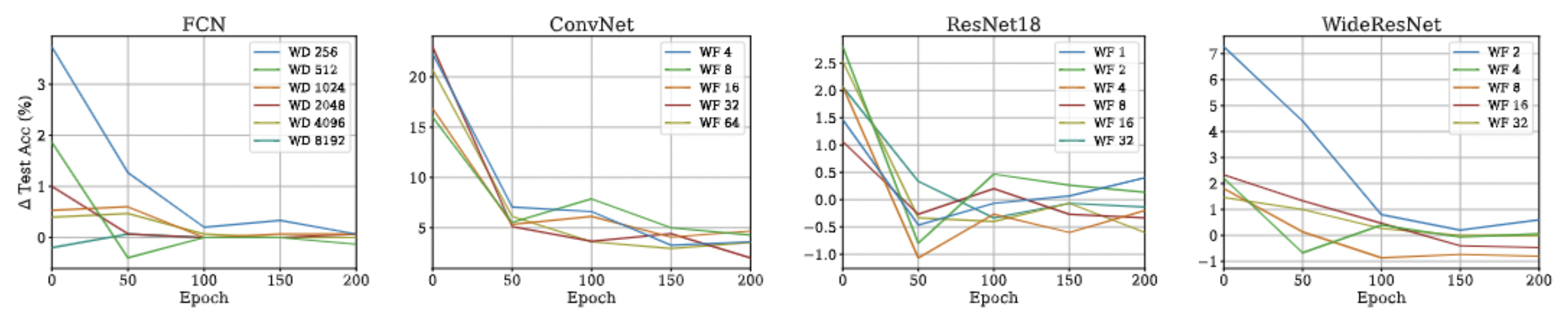
Approximation Quality: Kernel Regression

- Note: This approximation will not hold if there is any regularization (ridge) in the kernel regression! :(
- Note that we are not scaling the function values anymore!
Approximation Quality: Kernel Regression