CS6910: Fundamentals of Deep Learning
Lecture 7: Autoencoders and relation to PCA, Regularization in autoencoders, Denoising autoencoders, Sparse autoencoders, Contractive autoencoders
Mitesh M. Khapra
Department of Computer Science and Engineering, IIT Madras
Module 7.1: Introduction to Autoencoders
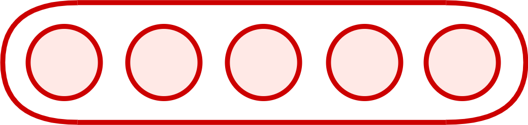
An autoencoder is a special type of feed forward neural network which does the following
Encodes its input \(\text x_ \text i\) into a hidden representation \(\text h\)
The model is trained to minimize a certain loss function which will ensure that \(\hat \text{x}_\text{i}\) is close to \(\text{x}_\text i\) (we will see some such loss functions soon)
Decodes the input again from this hidden representation
\(\hat \text{x}_\text{i}\)
\(\text{x}_\text{i}\)
\(\ \text{h}\)
\(W^*\)
\(W\)
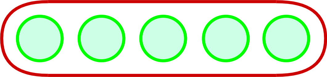
Let us consider the case where
\(\text {dim}\)(\(\textbf h) < \text {dim} (\textbf x_ \textbf i)\)
If we are still able to reconstruct \(\hat \text{x}_\text{i}\) perfectly from \(\text h\), then what does it say about \(\text h\)?
Do you see an analogy with PCA?
\(\text h\) is a loss-free encoding of \(\text{x}_\text i\). It captures all the important characteristics of \(\text{x}_\text i\)
\(\hat \text{x}_\text{i}\)
\(\text{x}_\text{i}\)
\(\ \text{h}\)
\(W^*\)
\(W\)
An autoencoder where \(\text {dim}\)(\(\textbf h) < \text {dim} (\textbf x_ \textbf i)\) is called an under complete autoencoder
In such a case the autoencoder could learn a trivial encoding by simply copying \(\text{x}_\text{i}\) into \(\text h\) and then copying \(\text h\) into \(\hat \text{x}_\text{i}\)
\(\hat \text{x}_\text{i}\)
\(\text{x}_\text{i}\)
\(\ \text{h}\)
\(W^*\)
\(W\)
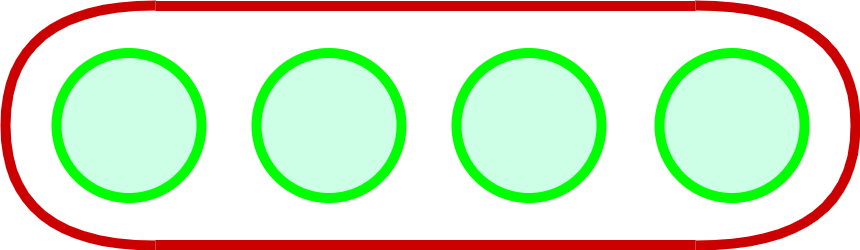
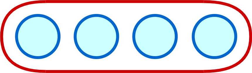
Let us consider the case where
\(\text {dim}\)(\(\textbf h) \ge \text {dim} (\textbf x_ \textbf i)\)
Let us consider the case where
\(\text {dim}\)(\(\textbf h) \ge \text {dim} (\textbf x_ \textbf i)\)
In such a case the autoencoder could learn a trivial encoding by simply copying \(\text{x}_\text{i}\) into \(\text h\) and then copying \(\text h\) into \(\hat \text{x}_\text{i}\)
\(\hat \text{x}_\text{i}\)
\(\text{x}_\text{i}\)
\(\ \text{h}\)
\(W^*\)
\(W\)
Do you see an analogy with PCA?
Such an identity encoding is useless in practice as it does not really tell us anything about the important characteristics of the data
An autoencoder where \(\text {dim}\)(\(\textbf h) \geq \text {dim} (\textbf x_ \textbf i)\) is called an over complete autoencoder
The Road Ahead
Choice of \(f(\textbf x_ \textbf i)\) and \(g(\textbf x_ \textbf i)\)
Choice of loss function
The Road Ahead
Choice of \(f(\textbf x_ \textbf i)\) and \(g(\textbf x_ \textbf i)\)
Choice of loss function
\(\text{x}_\text{i}\)
\(W^*\)
\(W\)
\(0\)
\(1\)
\(1\)
\(0\)
\(1\)
(binary inputs)
Suppose all our inputs are binary (each \(x_{ij} \in {0,1}\))
Which of the following functions would be most apt for the decoder?
Logistic as it naturally restricts all
outputs to be between 0 and 1
\(g\) is typically chosen as the sigmoid function
\(\text{x}_\text{i}\)
\(W^*\)
\(W\)
\(0.25\)
\(0.5\)
\(1.25\)
\(3.5\)
\(4.5\)
(real valued inputs)
Suppose all our inputs are real (each \(x_{ij} \in \mathbb R\))
Which of the following functions would be most apt for the decoder?
What will logistic and tanh do?
Again, \(g\) is typically chosen as the sigmoid function
They will restrict the reconstructed \(\hat \text{x}_\text{i}\) to lie between \([0,1]\) or \([-1,1]\) whereas we want \(\hat \text{x}_\text{i}\) \(\in \mathbb R^n\)
The Road Ahead
Choice of \(f(\textbf x_ \textbf i)\) and \(g(\textbf x_ \textbf i)\)
Choice of loss function
Consider the case when the inputs are real
valued
The objective of the autoencoder is to reconstruct ^xi to be as close to xi as possible
We can then train the autoencoder just like a regular feedforward network using back- propagation
This can be formalized using the following objective function:
\(\hat \text{x}_\text{i}\)
\(\text{x}_\text{i}\)
\(\ \text{h}\)
\(W^*\)
\(W\)
All we need is a formula for \(\frac{\partial \mathscr L(\theta)}{\partial W^*}\) and \(\frac{\partial \mathscr L(\theta)}{\partial W}\) which we will see now
Note that the loss function is shown for only one training example.
We have already seen how to calculate the expression in the boxes when we learnt backpropagation
\(h_2 = \hat \text{x}_\text{i}\)
\(h_0 = \text{x}_\text{i}\)
\(\text h_1\)
\(W^*\)
\(W\)
\(\text a_1\)
\(\text a_2\)
\(\text{x}_\text{i}\)
\(W^*\)
\(W\)
\(0\)
\(1\)
\(1\)
\(0\)
\(1\)
(binary inputs)
Consider the case when the inputs are binary
We use a sigmoid decoder which will produce outputs between 0 and 1, and can be interpreted as probabilities.
For a single n-dimensional \(i^{th}\) input we can use the following loss function
Again we need a formula for \(\frac{\partial \mathscr L(\theta)}{\partial W^*}\) and \(\frac{\partial \mathscr L(\theta)}{\partial W}\) to use backpropagation
What value of \(\hat x_{ij}\) will minimize this function?
If \(x_{ij} = 1 \) \(?\)
Indeed the above function will be minimized when \(\hat x_{ij} = x_{ij} !\)
If \(x_{ij} = 0 \) \(?\)
\(h_2 = \hat \text{x}_\text{i}\)
\(h_0 = \text{x}_\text{i}\)
\(\text h_1\)
\(W^*\)
\(W\)
\(\text a_1\)
\(\text a_2\)
We have already seen how to calculate the expressions in the square boxes when we learnt BP
The first two terms on RHS can be computed as:
Module 7.2: Link between PCA and Autoencoders
We will now see that the encoder part of an autoencoder is equivalent to PCA if we
use a linear encoder
use a linear decoder
use squared error loss function
normalize the inputs to
\(\hat \text{x}_\text{i}\)
\(\text{x}_\text{i}\)
\(\ \text{h}\)
\(\ \text{u}_1\)
\(\ \text{u}_2\)
\(\text x\)
\(\text y\)
PCA
\(P^TX^TXP = D\)
\(\equiv\)
First let us consider the implication of normalizing the inputs to
\(\hat \text{x}_\text{i}\)
\(\text{x}_\text{i}\)
\(\ \text{h}\)
\(P^TX^TXP = D\)
\(\equiv\)
The operation in the bracket ensures that the data now has \(0\) mean along each dimension \(j\) (we are subtracting the mean)
Let \(X'\) be this zero mean data matrix then what the above normalization gives us is \(X = \frac{1}{\sqrt m} X'\)
Now \((X)^TX = \frac{1}{\sqrt m} (X')^TX'\) is the covariance matrix (recall that covariance matrix plays an important role in PCA)
\(\ \text{u}_1\)
\(\ \text{u}_2\)
\(\text x\)
\(\text y\)
PCA
First we will show that if we use linear decoder and a squared error loss function then
\(\hat \text{x}_\text{i}\)
\(\text{x}_\text{i}\)
\(\ \text{h}\)
\(P^TX^TXP = D\)
\(\equiv\)
The optimal solution to the following objective function
is obtained when we use a linear encoder.
\(\ \text{u}_1\)
\(\ \text{u}_2\)
\(\text x\)
\(\text y\)
PCA
This is equivalent to
(just writing the expression (1) in matrix form and using the definition of \(\Vert A \Vert _ F\)) (we are ignoring the biases)
(1)
From SVD we know that optimal solution to the above problem is given by
By matching variables one possible solution is
We will now show that \(H\) is a linear encoding and nd an expression for the encoder weights \(W\)
Thus \(H\) is a linear transformation of \(X\) and \(W=V_{., \leq k}\)
We have encoder \(W=V_{., \leq k}\)
From SVD, we know that \(V\) is the matrix of eigen vectors of \(X^TX\)
From PCA, we know that P is the matrix of the eigen vectors of the covariance matrix
We saw earlier that, if entries of \(X\) are normalized by
then \(X^TX\) is indeed the covariance matrix
Thus, the encoder matrix for linear autoencoder (\(W\)) and the projection
matrix (\(P\)) for PCA could indeed be the same. Hence proved
Remember
The encoder of a linear autoencoder is equivalent to PCA if we
use a linear encoder
use a linear decoder
use a squared error loss function
and normalize the inputs to
Module 7.3: Regularization in autoencoders (Motivation)
Here, (as stated earlier) the model can simply learn to copy \(\text{x}_\text{i}\) into \(\text h\) and then copying \(\text h\) into \(\hat \text{x}_\text{i}\)
\(\hat \text{x}_\text{i}\)
\(\text{x}_\text{i}\)
\(\ \text{h}\)
\(W^*\)
\(W\)
While poor generalization could happen even in undercomplete autoencoders it is an even more serious problem for overcomplete auto encoders
To avoid poor generalization, we need to introduce regularization
The simplest solution is to add a L2-regularization term to the objective function
This is very easy to implement and just adds a term \(\lambda W\) to the gradient \(\frac{\partial \mathscr L(\theta)}{\partial W}\) (and similarly for other parameters)
\(\hat \text{x}_\text{i}\)
\(\text{x}_\text{i}\)
\(\ \text{h}\)
\(W^*\)
\(W\)
Another trick is to tie the weights of the encoder and decoder
This effectively reduces the capacity of Autoencoder and acts as a regularizer
\(\hat \text{x}_\text{i}\)
\(\text{x}_\text{i}\)
\(\ \text{h}\)
\(W^*\)
\(W\)
i.e., \(W^* = W^T\)
Module 7.4: Denoising Autoencoders
A denoising encoder simply corrupts the input data using a probabilistic process (\(P(\tilde x_{ij}|x_{ij})\)) before feeding it to the network
A simple \(P(\tilde x_{ij}|x_{ij})\) used in practice is the following
\(\hat \text{x}_\text{i}\)
\(\tilde \text{x}_\text{i}\)
\(\ \text{h}\)
\(P(\tilde x_{ij}|x_{ij})\)
\(\text{x}_\text{i}\)
In other words, with probability \(q\) the input is flipped to \(0\) and with probability \((1-q)\) it is retained as it is
How does this help ?
It no longer makes sense for the model to copy the corrupted \(\tilde \textbf x_i\) into \(h(\tilde \textbf x_i)\) and then into \(\tilde \textbf x_i\) (the objective function will not be minimized by doing so)
This helps because the objective is still to reconstruct the original (uncorrupted) \(\textbf x_i\)
Instead the model will now have to capture the characteristics of the data correctly.
For example, it will have to learn to reconstruct a corrupted \(x_{ij}\) correctly by relying on its interactions with other elements of \(x_i\)
\(\hat \text{x}_\text{i}\)
\(\tilde \text{x}_\text{i}\)
\(\ \text{h}\)
\(P(\tilde x_{ij}|x_{ij})\)
\(\text{x}_\text{i}\)
We will now see a practical application in which AEs are used and then compare Denoising Autoencoders with regular autoencoders
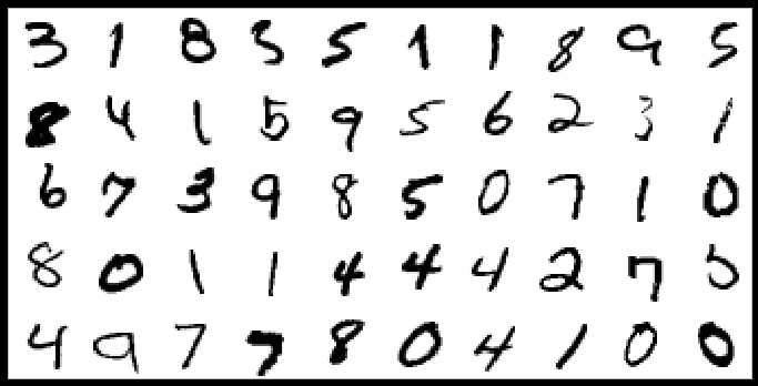
Task: Hand-written digit
recognition
Figure: MNIST Data
Figure: Basic approach (we use raw data as input features)
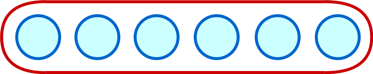
\(0\)
\(1\)
\(2\)
\(3\)
\(9\)
\(|\textbf x_{i}| = 784 = 28 \times 28\)
\(28 * 28\)
\(0\)
\(1\)
\(2\)
\(3\)
\(9\)
Task: Hand-written digit
recognition
Figure: AE approach (first learn important
characteristics of data)
\(|\textbf x_{i}| = 784 = 28 \times 28\)
\(28 * 28\)
Figure: MNIST Data
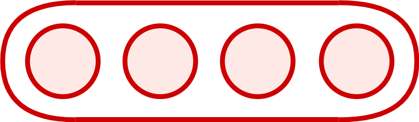
\(\textbf h \in \mathbb R^d\)
\(\hat \textbf x_i \in \mathbb R^{784}\)
Task: Hand-written digit
recognition
Figure: AE approach (and then train a classifier on top of this hidden representation)
\(|\textbf x_{i}| = 784 = 28 \times 28\)
\(28 * 28\)
\(\textbf h \in \mathbb R^d\)
Figure: MNIST Data
\(0\)
\(1\)
\(2\)
\(3\)
\(9\)
\(0\)
\(1\)
\(2\)
\(3\)
\(9\)
We will now see a way of visualizing AEs and use this visualization to compare different AEs
We can think of each neuron as a lter which will re (or get maximally) activated for a certain input con guration \(\textbf x_i\)
For example,
Where \(W_1\) is the trained vector of weights connecting the input to the first hidden neuron
What values of \(\textbf x_i\) will cause \(\textbf h_1\) to be maximum (or maximally activated)
Suppose we assume that our inputs are normalized so that \(\Vert \textbf x_i \Vert =1\)
\( \max \limits_{\textbf x_i} \{ W_1^T \textbf x_i\}\)
\(s.t.\) \(\Vert \textbf x_i \Vert ^2 \) \(= \textbf x_i ^T \textbf x_i = 1 \)
\(\hat \text{x}_\text{i}\)
\(\text{x}_\text{i}\)
\(\ \text{h}\)
Solution: \(\textbf x_i = \cfrac{W_1}{\sqrt {W_1^TW_1}}\)
Thus the inputs
will respectively cause hidden neurons \(1\) to \(n\) to maximally fire
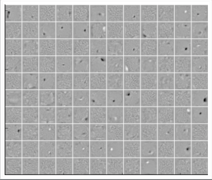
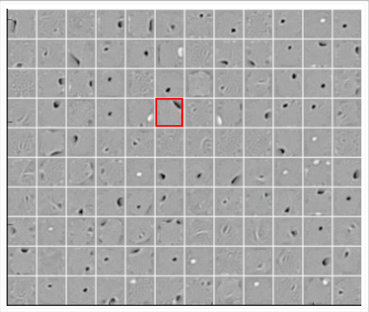
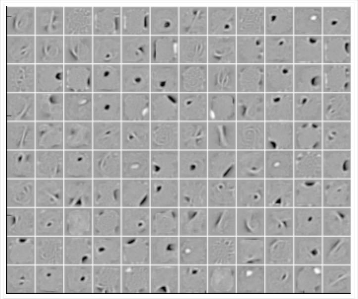
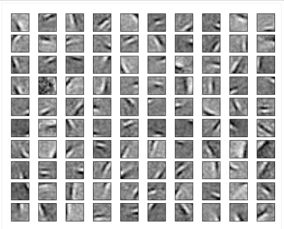
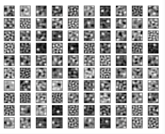
Let us plot these images (\(\textbf x_i\)'s) which maximally activate the first \(k\) neurons of the hidden representations learned by a vanilla autoencoder and different denoising autoencoders
These \(\textbf x_i\)'s are computed by the above formula using the weights \((W_1, W_2 ... W_k)\) learned by the respective autoencoders
\( \max \limits_{\textbf x_i} \{ W_1^T \textbf x_i\}\)
\(s.t.\) \(\Vert \textbf x_i \Vert ^2 \) \(= \textbf x_i ^T \textbf x_i = 1 \)
\(\hat \text{x}_\text{i}\)
\(\text{x}_\text{i}\)
\(\ \text{h}\)
Solution: \(\textbf x_i = \cfrac{W_1}{\sqrt {W_1^TW_1}}\)
The vanilla AE does not learn many meaningful patterns
The hidden neurons of the denoising AEs seem to act like pen-stroke detectors (for example, in the highlighted neuron the black region is a stroke that you would expect in a '0' or a '2' or a '3' or a '8' or a '9')
As the noise increases the filters become more wide because the neuron has to rely on more adjacent pixels to feel confident about a stroke
Figure: Vanilla AE
(No noise)
Figure: 25% Denoising
AE (q=0.25)
Figure: 50% Denoising
AE (q=0.5)
We saw one form of \(P(\tilde x_{ij}|x_{ij})\) which flips a fraction \(q\) of the inputs to zero
\(\hat \text{x}_\text{i}\)
\(\tilde \text{x}_\text{i}\)
\(\ \text{h}\)
\(P(\tilde x_{ij}|x_{ij})\)
\(\text{x}_\text{i}\)
Another way of corrupting the inputs is to add
a Gaussian noise to the input
\(\tilde x_{ij} = x_{ij} + \mathcal N (0,1)\)
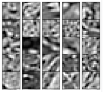
We will now use such a denoising AE on a different dataset and see their performance
The hidden neurons essentially behave like edge detectors
PCA does not give such edge detectors
Figure: Data
Figure: AE filters
Figure: Weight decay filters
Module 7.5: Sparse Autoencoders
\(\hat \text{x}_\text{i}\)
\(\text{x}_\text{i}\)
\(\ \text{h}\)
\(W^*\)
\(W\)
A hidden neuron with sigmoid activation will have values between 0 and 1
We say that the neuron is activated when its output is close to 1 and not activated when its output is close to 0.
A sparse autoencoder tries to ensure the neuron is inactive most of the times.
\(\hat \text{x}_\text{i}\)
\(\text{x}_\text{i}\)
\(\ \text{h}\)
\(W^*\)
\(W\)
If the neuron \(l\) is sparse (i.e. mostly inactive) then \(\hat \rho _l \rightarrow 0\)
A sparse autoencoder uses a sparsity parameter \(\rho\) (typically very close to 0, say, 0.005) and tries to enforce the constraint \(\hat \rho_l = \rho\)
One way of ensuring this is to add the following term to the objective function
When will this term reach its minimum value and what is the minimum value? Let us plot it and check.
The average value of the activation of a neuron \(l\) is given by
The function will reach its minimum value(s) when \(\hat \rho_l = \rho\).

\(\hat \rho_l\)
\(\Omega (\theta) \)
\(0.2\)
\(\rho = 0.2\)
Now,
\(\hat \mathscr L (\theta) = \mathscr L (\theta) + \Omega (\theta) \)
\(\mathscr L (\theta)\) is the squared error loss or cross entropy loss and \(\Omega (\theta)\) is the sparsity constraint.
We already know how to calculate \(\frac{\partial \mathscr L (\theta)}{\partial W}\)
Let us see how to calculate \(\frac{\partial \mathscr \Omega (\theta)}{\partial W}\)
Finally,
(and we know how to calculate both terms on R.H.S)
Can be re-written as
By Chain rule:
For each neuron \(l \in 1...k\) in hidden layer, we have
(see next slide)
and
Derivation
For each element in the above equation we can calculate \(\frac{\partial \hat \rho_l}{\partial W}\) (which is the partial derivative of a scalar w.r.t. a matrix = matrix). For a single element of a matrix \(W_{jl}\):-
So in matrix notation we can write it as :
Module 7.6: Contractive Autoencoders
A contractive autoencoder also tries to prevent an overcomplete autoencoder from learning the identity function.
It does so by adding the following regularization term to the loss function
\(\hat \text{x}\)
\(\text{x}\)
\(\ \text{h}\)
\(W^*\)
\(W\)
where, \(J_\textbf x (\textbf h)\) is the Jacobian of the encoder.
Let us see how it looks like.
If the input has \(n\) dimensions and the hidden layer has \(k\) dimensions then
In other words, the (\(j, l\)) entry of the Jacobian captures the variation in the output of the \(l^{th}\) neuron with a small variation in the \(j^{th}\) input.
What is the intuition behind this ?
Consider \(\frac{\partial h_1}{\partial x_1}\), what does it mean if \(\frac{\partial h_1}{\partial x_1} = 0\) ?
It means that this neuron is not very sensitive to variations in the input \(x_1\).
But doesn't this contradict our other goal of minimizing \(\mathscr L (\theta)\) which requires \(\mathbf h\) to capture variations in the input.
\(\hat \text{x}_\text{i}\)
\(\text{x}_\text{i}\)
\(\ \text{h}\)
Indeed it does and that's the idea
By putting these two contradicting objectives against each other we ensure that \(h\) is sensitive to only very important variations as observed in the training data.
Tradeoff - capture only very important variations in the data
\(\mathscr L (\theta)\) - capture important variations in data
\(\hat \text{x}_\text{i}\)
\(\text{x}_\text{i}\)
\(\ \text{h}\)
\(\Omega(\theta)\) - do not capture variations in data
Let us try to understand this with the help of an illustration.
Consider the variations in the data along directions \(\mathbf u_1\) and \(\mathbf u_2\)
\(\ \text{u}_1\)
\(\ \text{u}_2\)
\(x\)
\(\text y\)
It makes sense to maximize a neuron to be sensitive to variations along \(\mathbf u_1\)
At the same time it makes sense to inhibit a neuron from being sensitive to variations along \(\mathbf u_2\) (as there seems to be small noise and unimportant for reconstruction)
What does this remind you of ?
By doing so we can balance between the contradicting goals of good reconstruction and low sensitivity.
Module 7.7: Summary
\(\hat \text{x}_\text{i}\)
\(\text{x}_\text{i}\)
\(\ \text{h}\)
\(\ \text{u}_1\)
\(\ \text{u}_2\)
\(\text x\)
\(\text y\)
PCA
\(P^TX^TXP = D\)
\(\equiv\)
\(\hat \text{x}_\text{i}\)
\(\tilde \text{x}_\text{i}\)
\(\ \text{h}\)
\(P(\tilde x_{ij}|x_{ij})\)
\(\text{x}_\text{i}\)
Regularization
Weight decaying
Sparse
Contractive