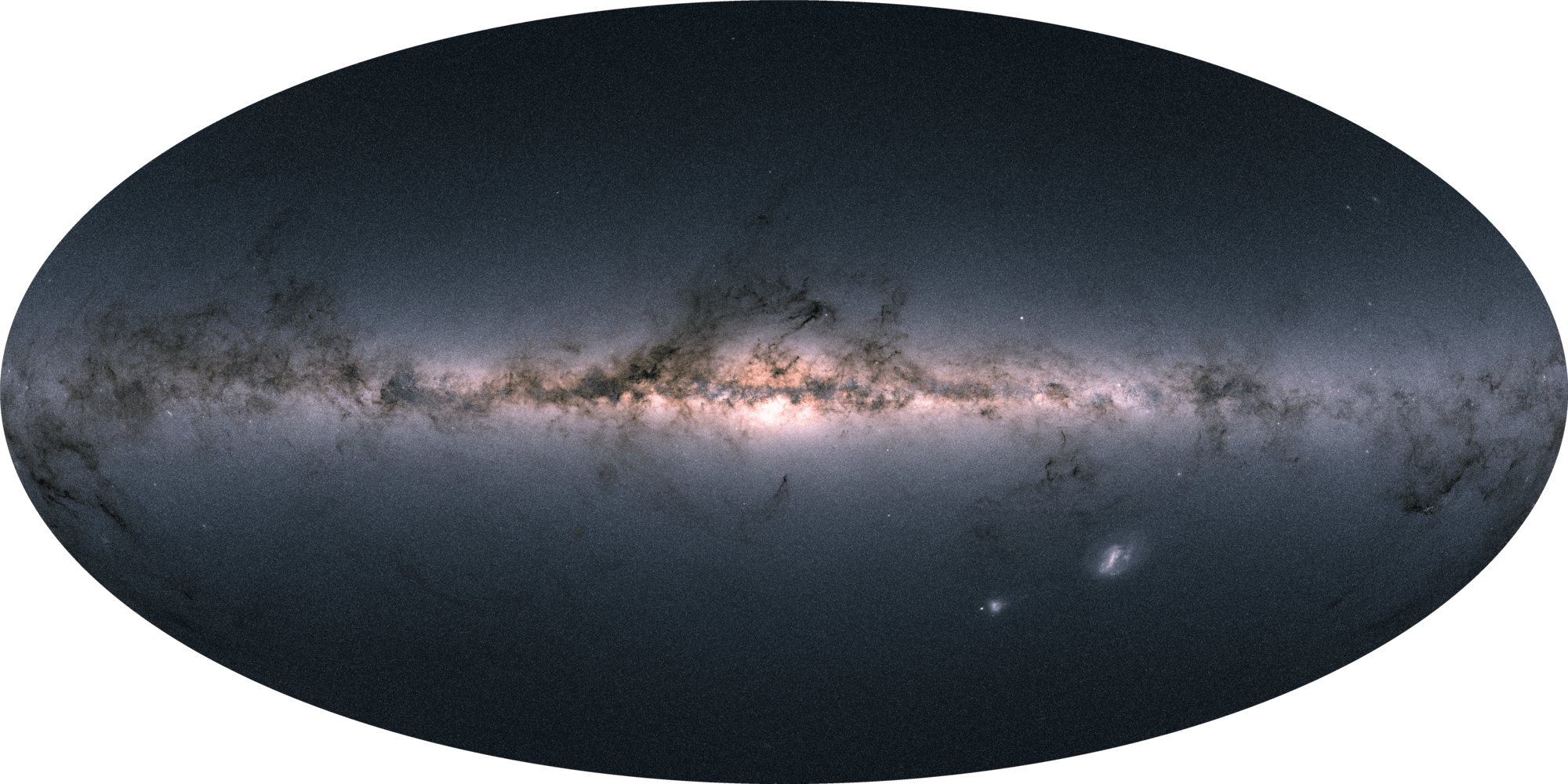

Image Credit: ESA
What are MS Dippers?
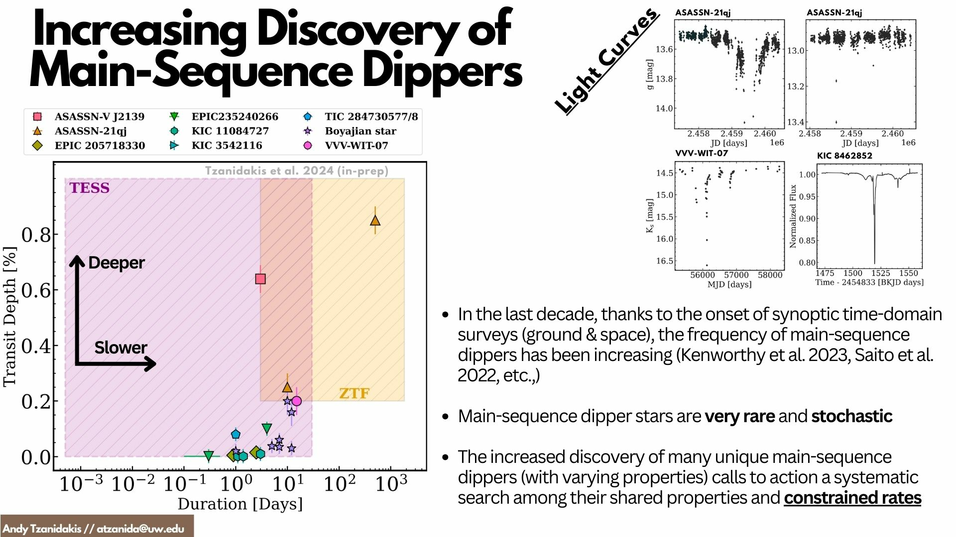
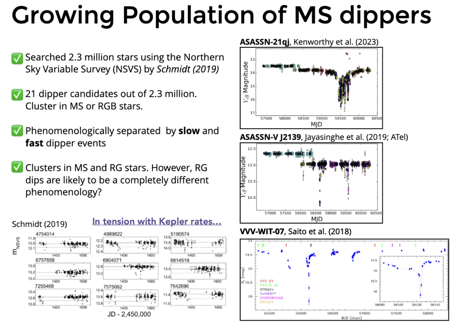
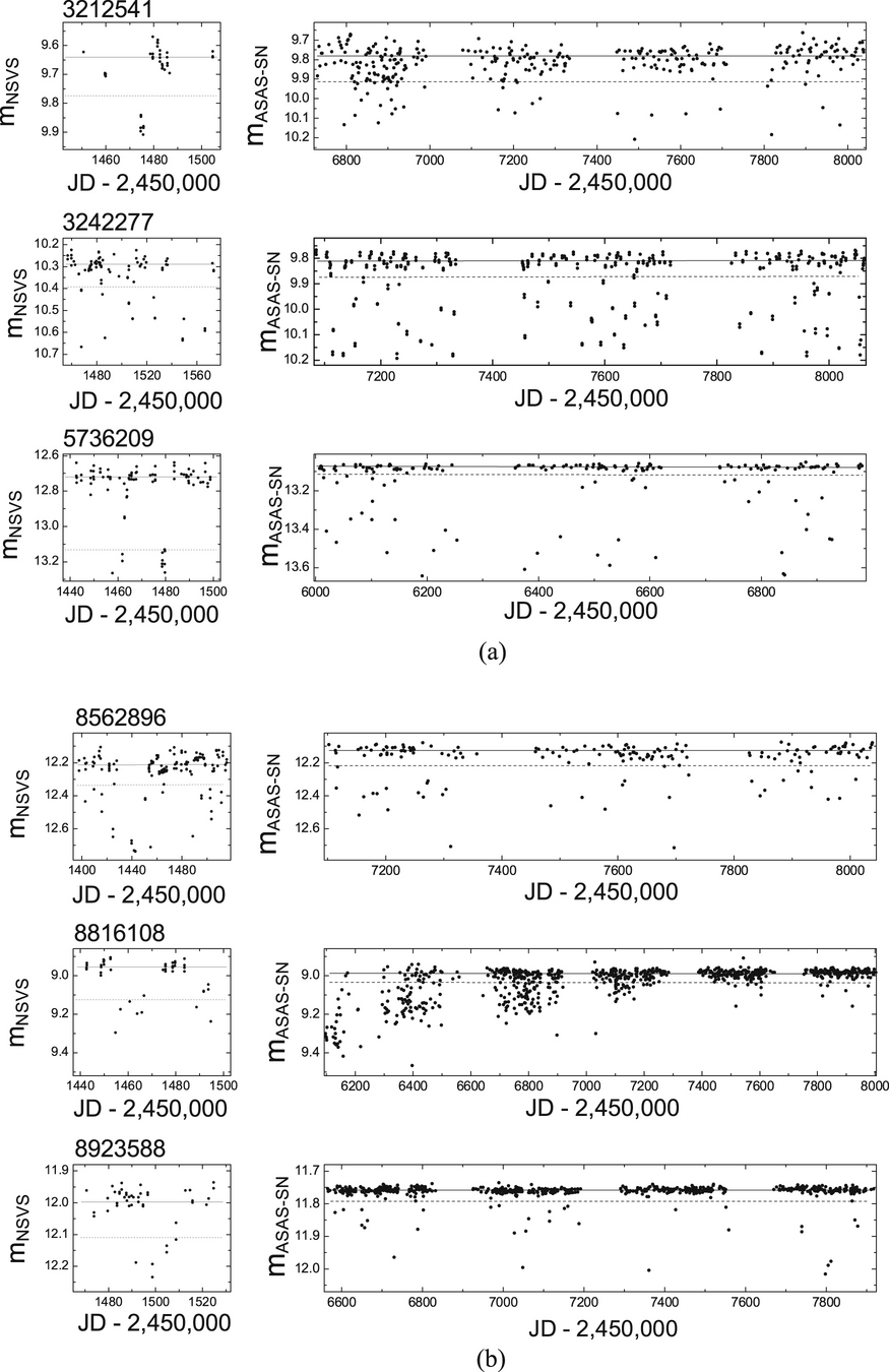
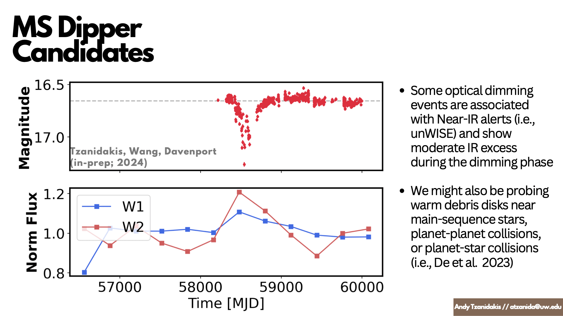
- Ordinary main-sequence (MS) stars that undergo complex and stochastic dimming events from hours to years...
- Kepler revealed that MS stars are quiescent with no complex stellar variability (Ciardi et al. 20211)
Kepler
Ciardi + 2011
-
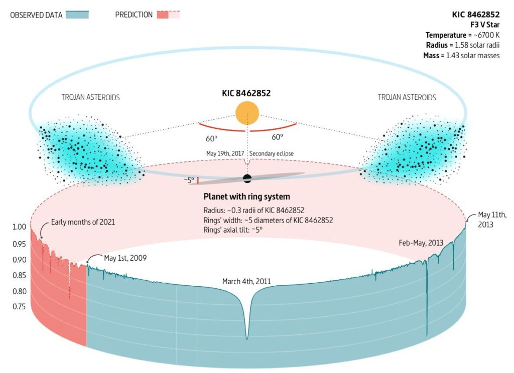
KIC 8462852 (Boyajian star), a main-sequence F0 dwarf that underwent large and complex dimmings (~1-7 days) that are hotly debated in the community (Boyajian et al. 2016, 2018)
-
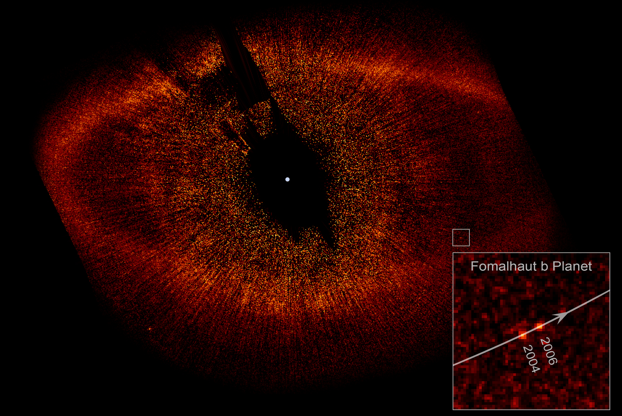
Several theories have been invoked, large comets (Boyajian +2016), trojan asteroids (Ballesteros +2017), planet-engulfment (Metgzer+2017), comet swarms (Makarov and Goldin 2016)
- The mechanism of the Boyajian star dimmings is not well constrained, except for signatures of possible sub-micron dust obscuring the primary star with no evidence of IR/mm excess
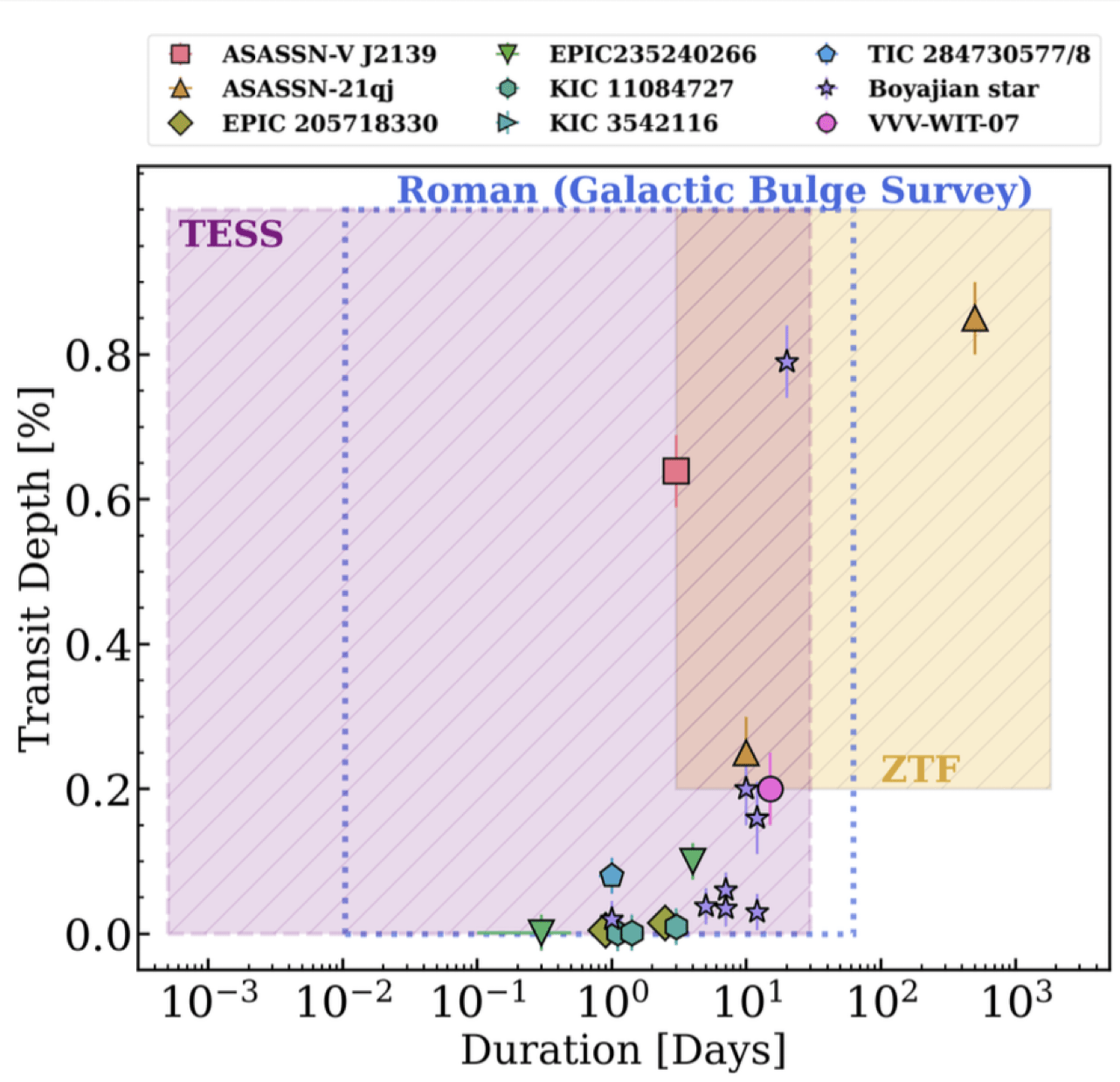
What is the Boyajian Star?
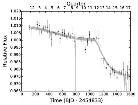
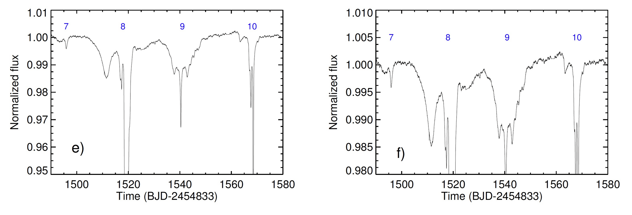
Deep and complex dimming (1-7 days)
No strong evidence for periodicity
Secular dimming ~0.1%
Not consistent with ISM reddening
Importance
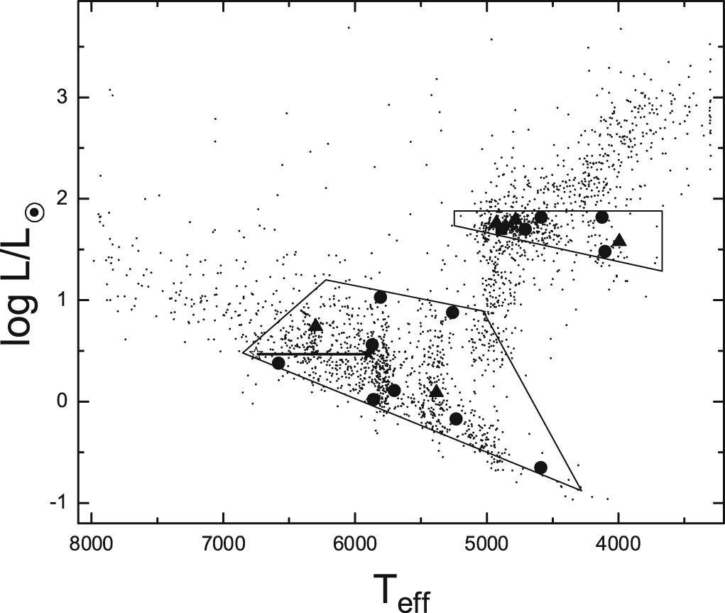
- The majority of Galactic stars are still within their main-sequence phase (Jurić et al. 2008)
- Important clues for Giant Impact Events and their effects on terrestrial planet formation (i.e., Quintana et al. 2016)
- Star-planet interactions and engulfment rates (i.e., Metzger et al. 2017)
- Debris disks and planetesimal interactions around MS stars (i.e., Hughes et al. 2022)
- Dynamics and configurations of interstellar comet swarms (i.e., Marakov and Goldin 2016)


NASA
NASA/JPL-Caltech
Ballesteros+2017
HST/JPL
We can do better...
poorly sampled EB's?! 🤨
On average ZTF covers ∼3750 square degrees per hour with a median limiting magnitude of r∼20.6 mag, g∼20.8 mag (Dekany et al. 2020; Bellm et al. 2019)
ZTF cadences typically span 1-3 day cadences with ~1-10% photometric precision
ZTF is a good TD survey to conduct a systematic search of Boyajian star analogs and searching techniques for LSST & Roman
Systematic Searches with ZTF and other Time-Domain Surveys
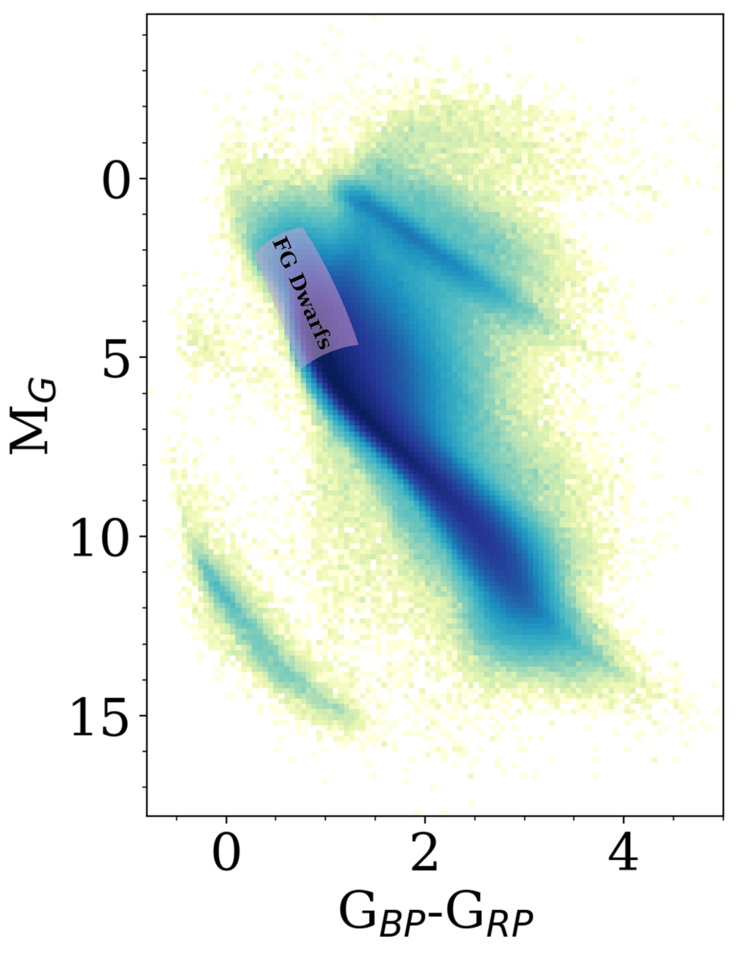
FGK Dwarfs
Large Systematic Search for MS Dippers
We are carrying out the first systematic search of ~60 million FGK MS stars
Gaia eDR3
ZTFubercal (Zubercal)
Stellar Parameters
Anders et al. 2022
Custom Cat.

Customizable Python time-series evaluation routines (e.g. fitting, time-series features, ...)
Zubercal (src)
Zubercal
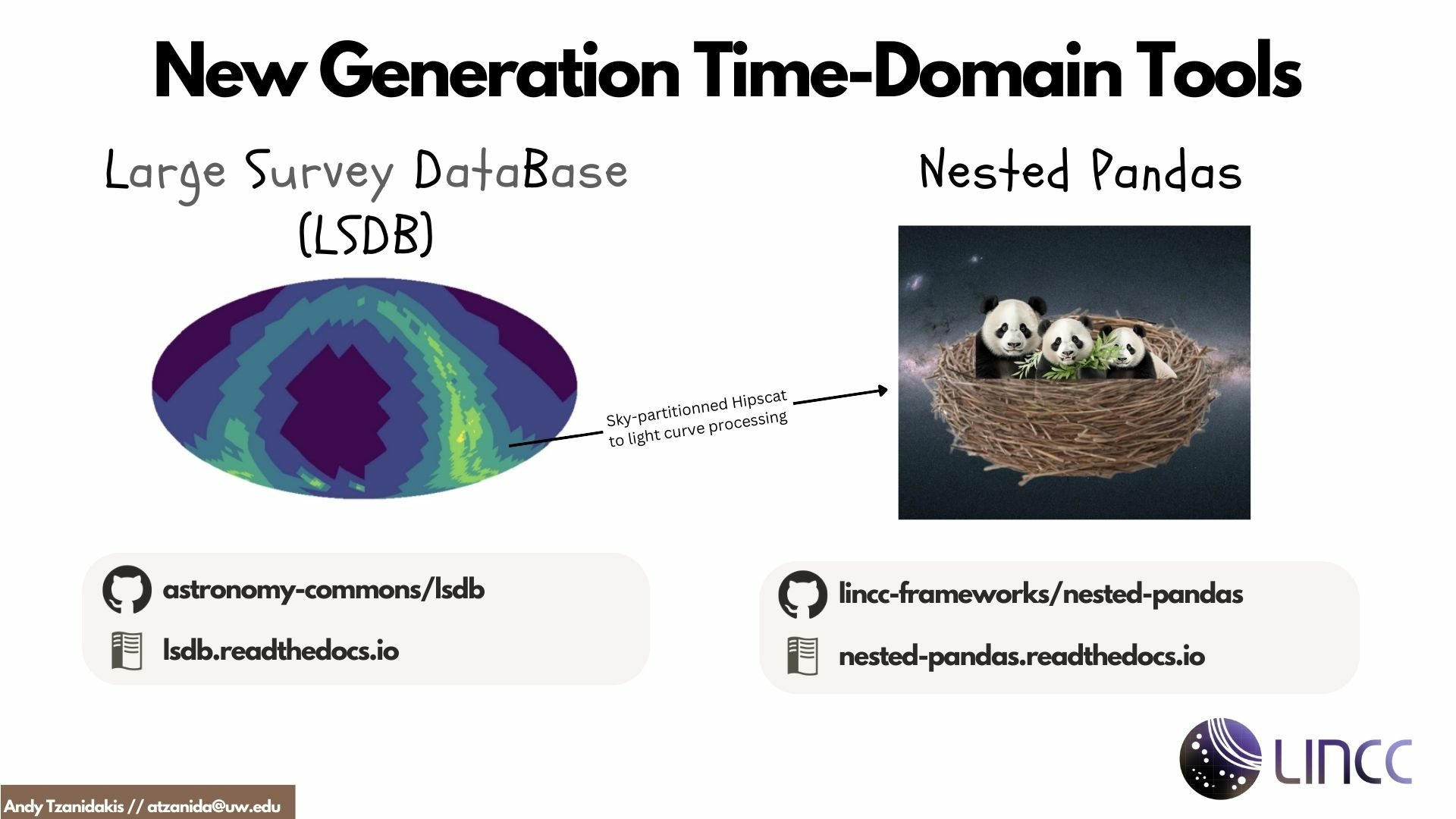
LSDB
Fast object catalog operations and querying
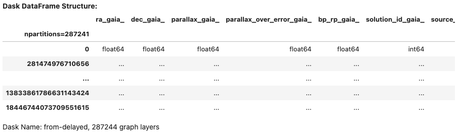
Nested DF
Bridges object
and source catalogs
Large Survey DataBase
Nested Pandas
Full ZTF DR14 Photometry
Identify Event
Scoring
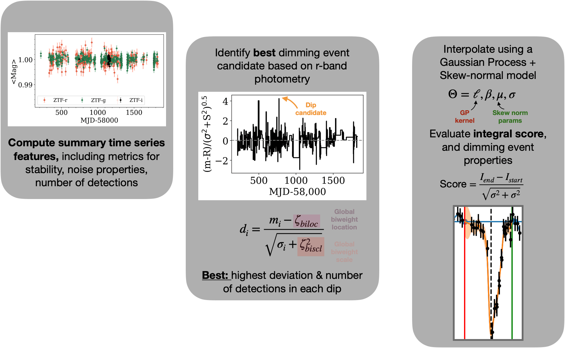
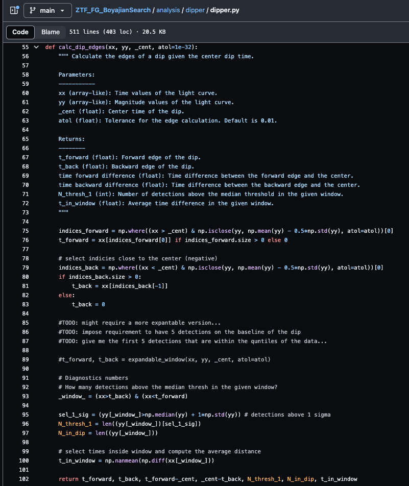
Dipper Pipeline
Tzanidakis et al. (2024; in-prep)
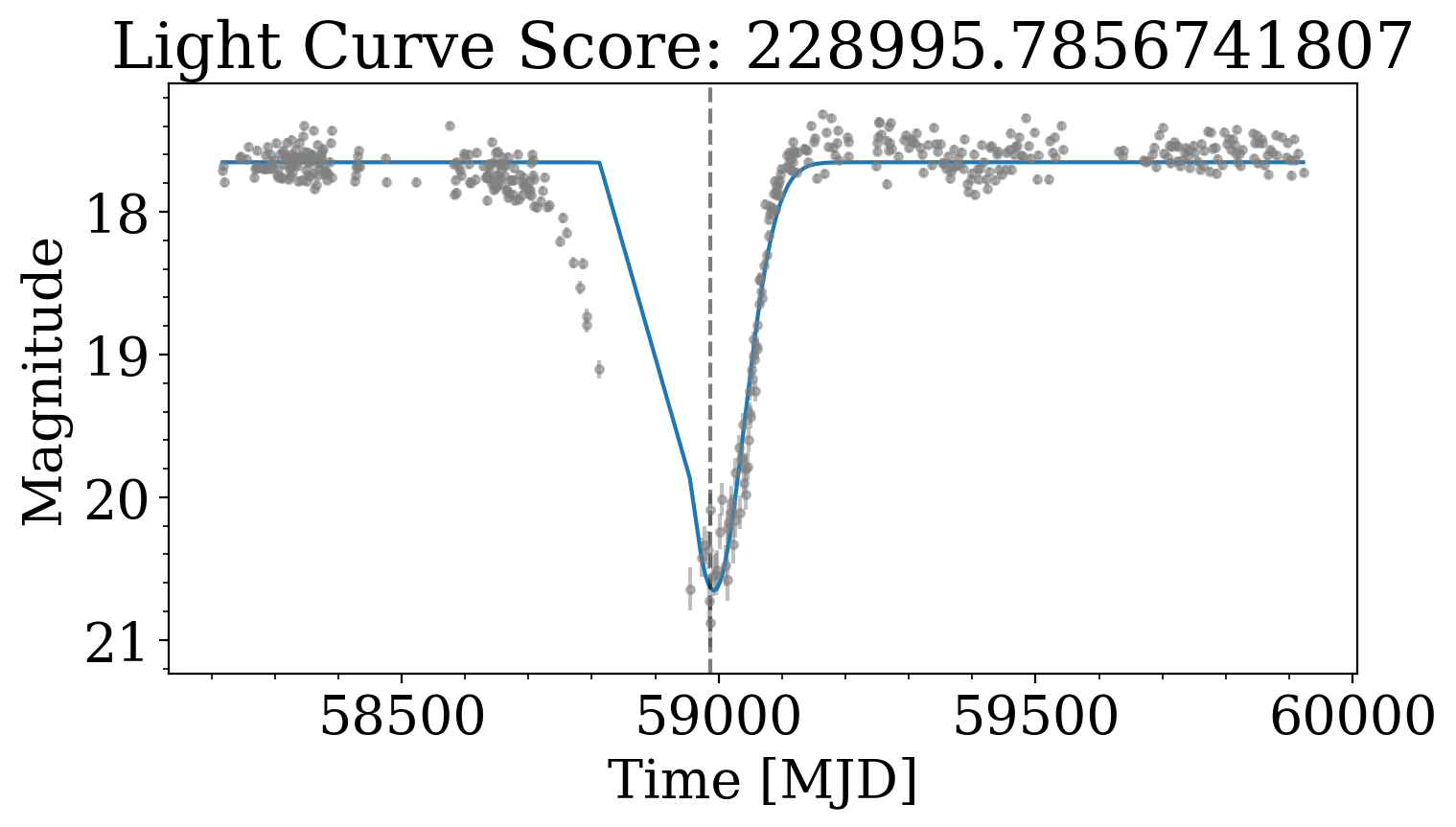
For each jth detected dip, we evaluate a Gaussian model, and compute the score for each dimming event.
Each light curve is ranked by dip amplitude, number of dips, scatter, and duration...
Peak finding algorithm
(Virtanen et al. 2020)
Score Distribution
Tzanidakis et al. (2024; in-prep)
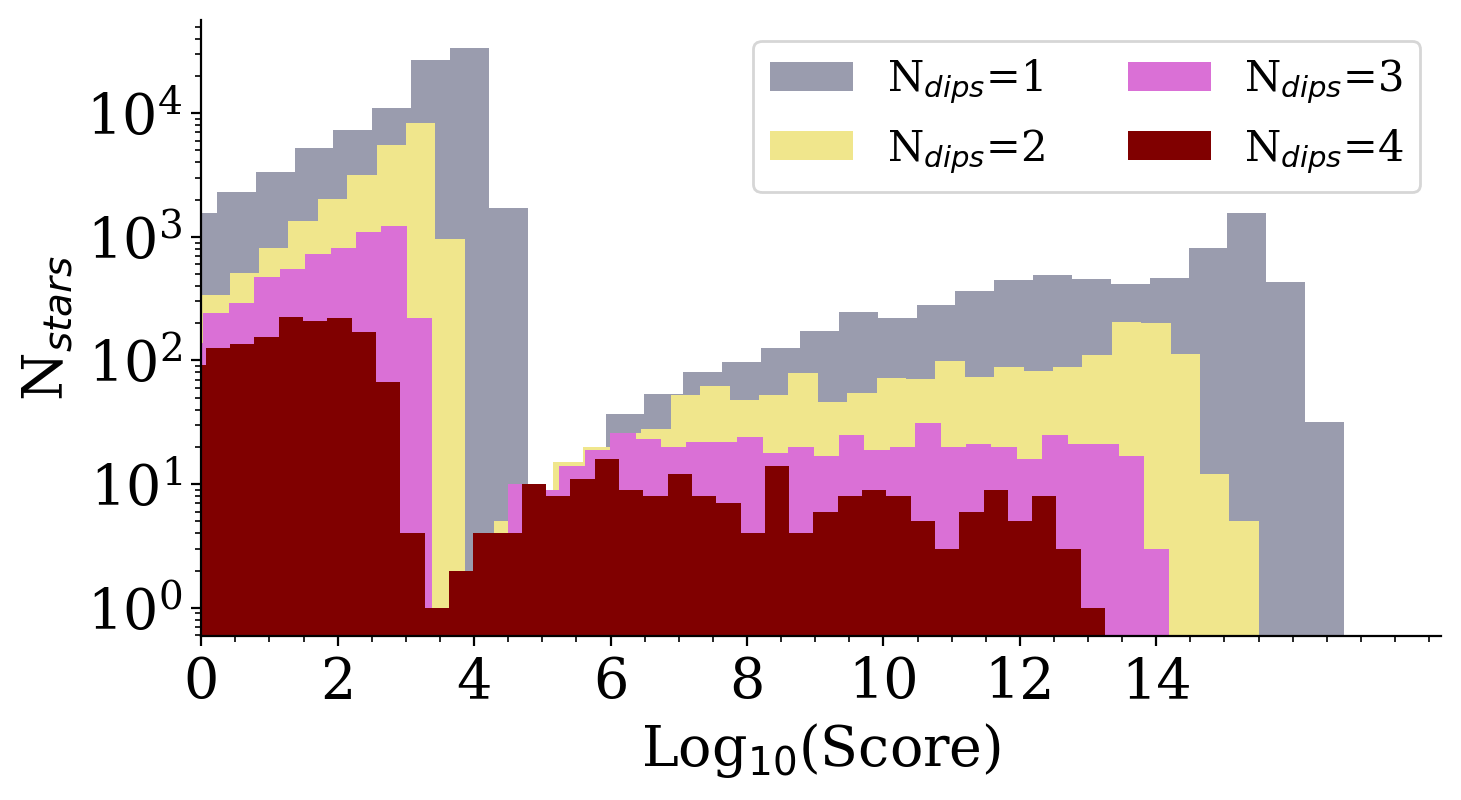
- Scoring algorithm is bimodal, making the separation and selection possibly easier...
- The score cut-off was determined based on injection-recovery tests to understand the
score limits of a dipper-like candidate (i.e., ~95% efficiency for Ndips=1)
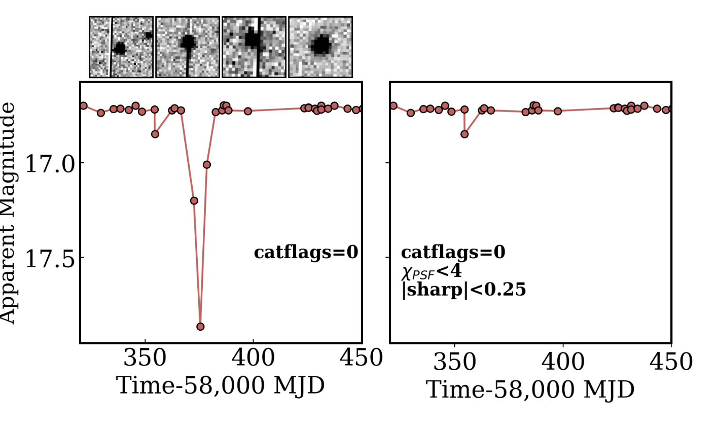
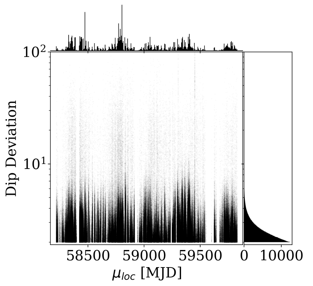
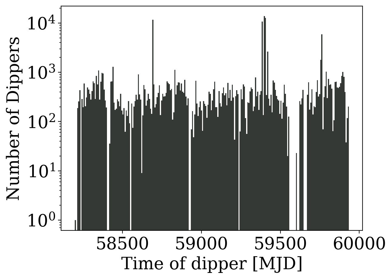
Sky Systematics
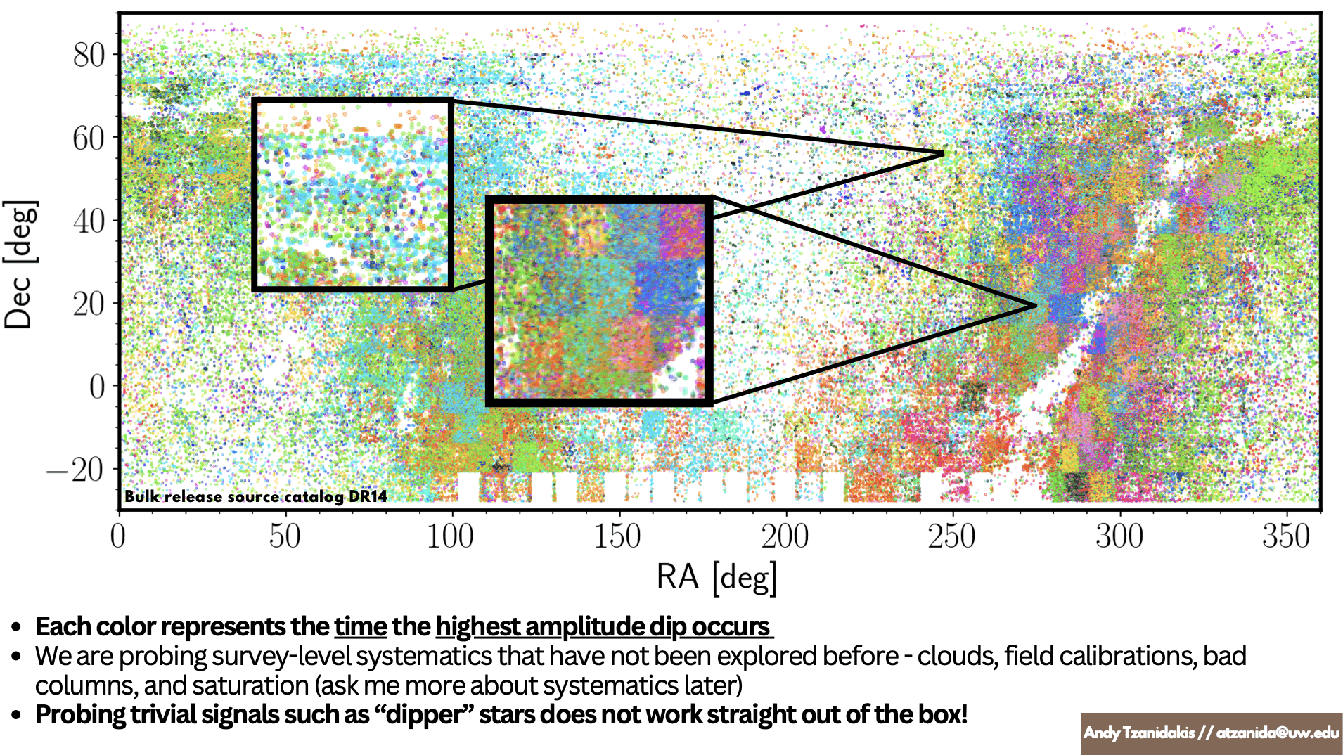
ZTF DR17
Tzanidakis et al. (2024; in-prep)
Sky Systematics
Zubercal
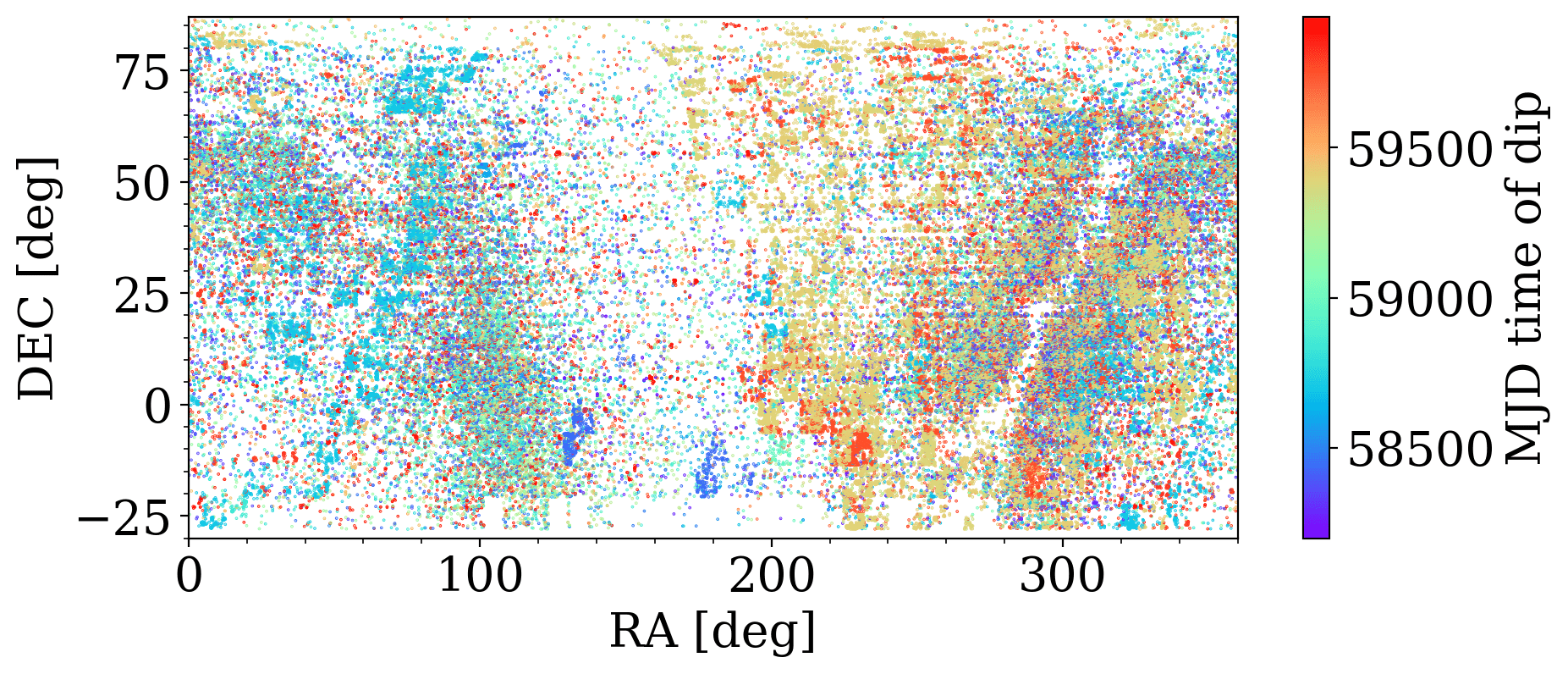
Tools like LSDB and Nested Pandas enable rapid assessment of survey wide systematics!
Tzanidakis et al. (2024; in-prep)
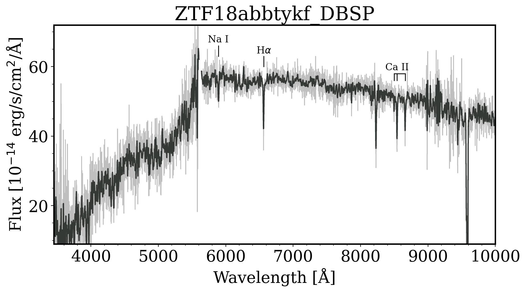
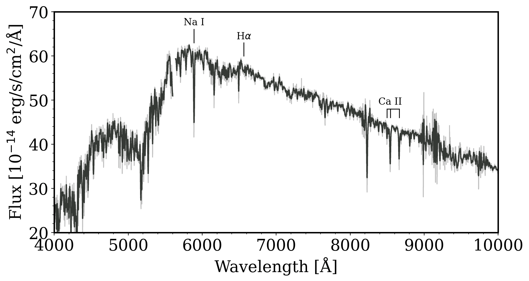
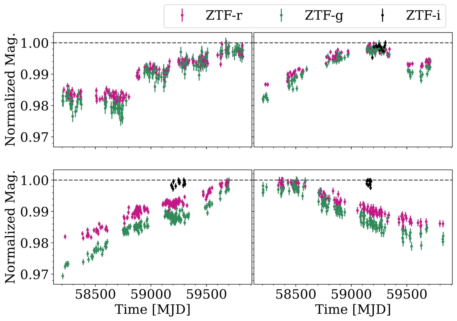
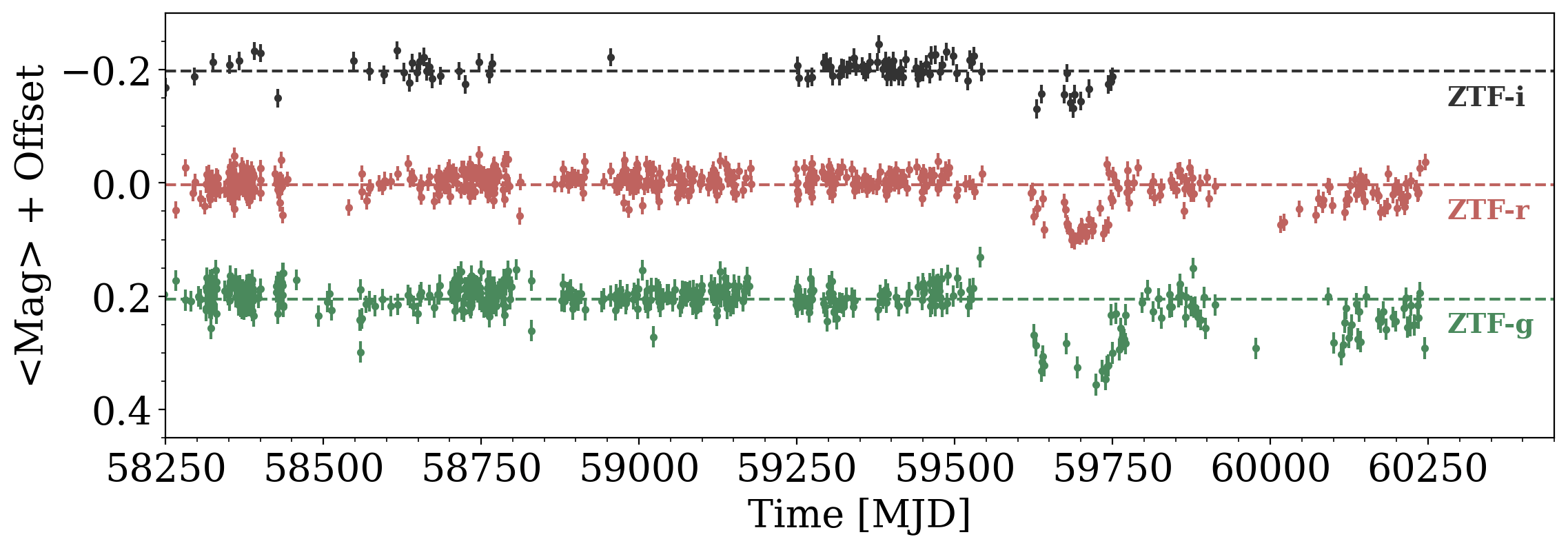
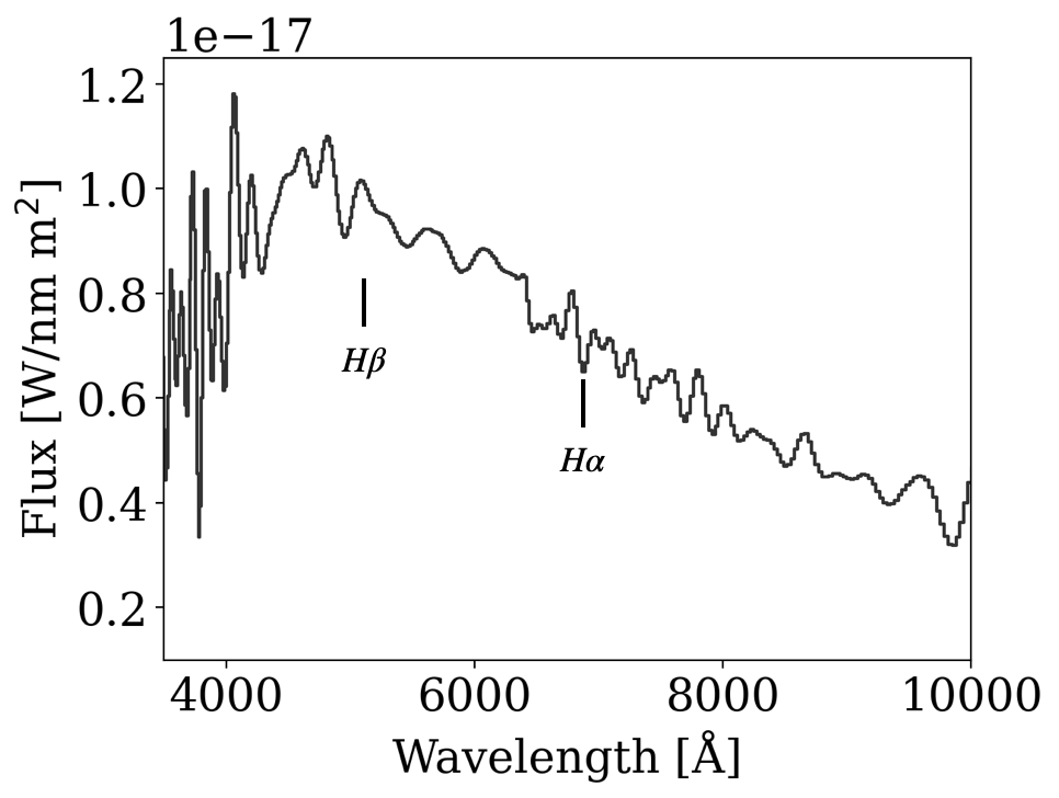
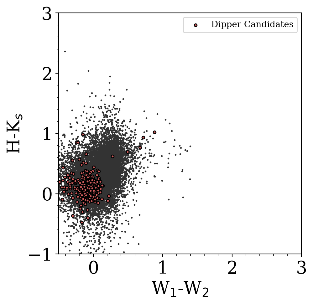
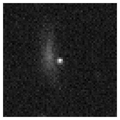
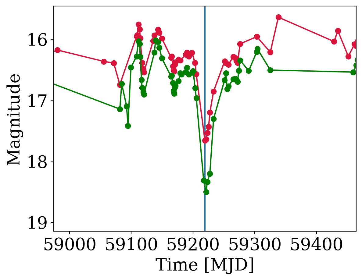
Main-Sequence Dipper Candidates
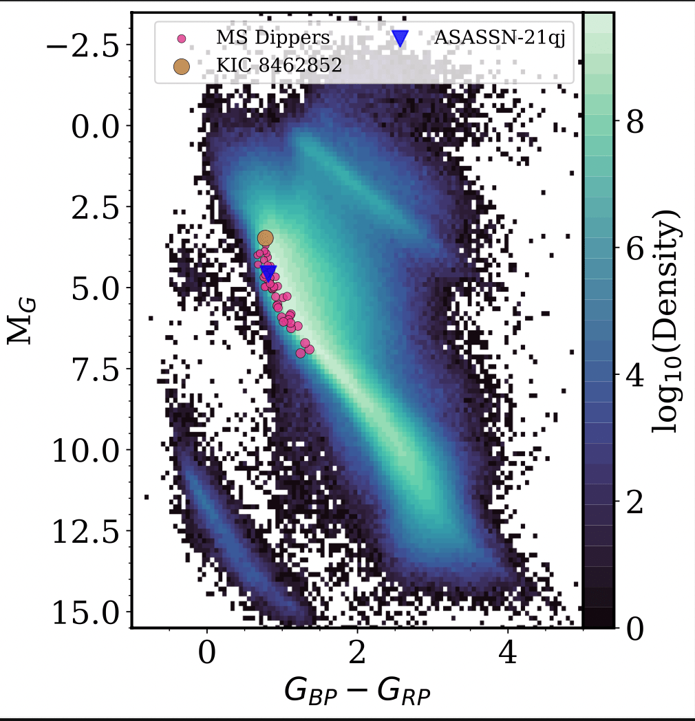
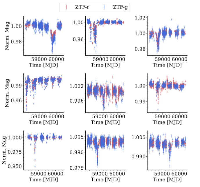
Tzanidakis et al. (2024; in-prep)
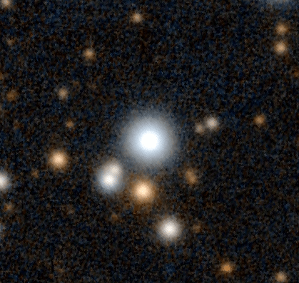
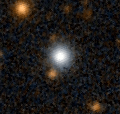
PS1 griz
PS1 griz
Tzanidakis et al. 2024 (in-prep)
DBSP, P200"
DBSP, P200"
Working with External Catalogs
catname = "I/354"
catalogue_ivoid = f"ivo://CDS.VizieR/{catname}"

# the actual query to the registry
voresource = registry.search(ivoid=catalogue_ivoid)[0]

voresource.describe(verbose=True)
StarHorse2, Gaia EDR3 photo-astrometric distances
Short Name: I/354
IVOA Identifier: ivo://cds.vizier/i/354
Access modes: conesearch, hips#hips-1.0, tap#aux, web
Multi-capabilty service -- use get_service()
We present a catalogue of 362 million stellar parameters, distances, and
extinctions derived from Gaia's Early Data Release (EDR3) cross-matched with
the photometric catalogues of Pan-STARRS1, SkyMapper, 2MASS, and AllWISE. The
higher precision of the Gaia EDR3 data, combined with the broad wavelength
coverage of the additional photometric surveys and the new stellar-density
priors of the StarHorse code, allows us to substantially improve the accuracy
and precision over previous photo-astrometric stellarparameter estimates. At
magnitude G=14 (17), our typical precisions amount to 3% (15%) in distance,
0.13mag (0.15mag) in V-band extinction, and 140K (180K) in effective
temperature. Our results are validated by comparisons with open clusters, as
well as with asteroseismic and spectroscopic measurements, indicating
systematic errors smaller than the nominal uncertainties for the vast majority
of objects. We also provide distance- and extinction-corrected colour-
magnitude diagrams, extinction maps, and extensive stellar density maps that
reveal detailed substructures in the Milky Way and beyond. The new density
maps now probe a much greater volume, extending to regions beyond the Galactic
bar and to Local Group galaxies, with a larger total number density. We
publish our results through an ADQL query interface (gaia.aip.de) as well as
via tables containing approximations of the full posterior distributions. Our
multi-wavelength approach and the deep magnitude limit render our results
useful also beyond the next Gaia release, DR3.
Subjects: I/354
Waveband Coverage:
More info: https://cdsarc.cds.unistra.fr/viz-bin/cat/I/354# execute a synchronous ADQL query
tap_service = voresource.get_service("tap")
# Function to run a TAP query and return a Dask DataFrame
def query_tap(service, ra_min, ra_max, dec_min, dec_max):
query = f'''
SELECT *
FROM "{first_table_name}"
WHERE ra BETWEEN {ra_min} AND {ra_max}
AND dec BETWEEN {dec_min} AND {dec_max}
'''
tap_records = service.run_sync(query)
tbl = tap_records.to_table()
df = tbl.to_pandas()
return dd.from_pandas(df, npartitions=1)
# Initialize the Dask DataFrame
final_ddf = dd.DataFrame()
# Coordinate limits
ra_min, ra_max = 0, 360
dec_min, dec_max = -30, 90
# Service initialization (replace with actual service initialization)
service = voresource.get_service("tap")
# Perform the queries in chunks and append to the Dask DataFrame
for dec in range(dec_min, dec_max, dec_step):
dec_min_chunk, dec_max_chunk = dec, dec+dec_step
chunk_ddf = query_tap(service, ra_min, ra_max, dec_min_chunk, dec_max_chunk)
# Concatenate the new chunk with the final Dask DataFrame
if final_ddf.npartitions == 0:
final_ddf = chunk_ddf
else:
final_ddf = dd.concat([final_ddf, chunk_ddf])VizieR:
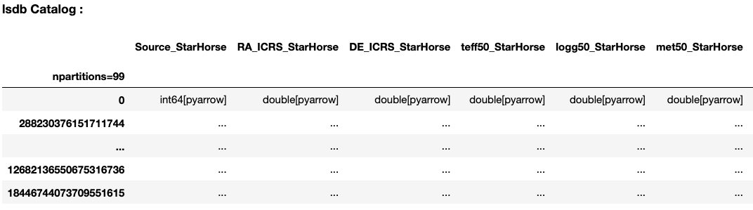
Query & clean object table
from hipscat_import.catalog.arguments import ImportArguments
args = ImportArguments(
ra_column="RA_ICRS_StarHorse",
dec_column="DE_ICRS_StarHorse",
file_reader="parquet",
input_file_list=[f"{input_file}"],
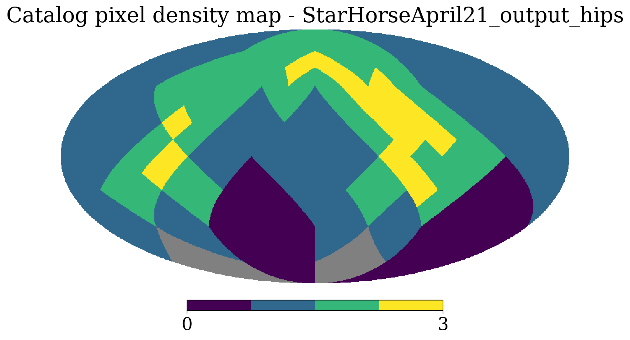
output_artifact_name="StarHorseApril21_output_hips",
output_path="/nvme/users/atzanida/tmp/",
resume=False,
)LSDB Workflow
Hipscat via `ImportArguments`
Hipscat
sky partitions
order
Nested Pandas Workflow
# load StarHorse table
object_table = lsdb.read_hipscat("/nvme/users/atzanida/tmp/StarHorseApril21_output_hips")

# Load ZTF DR17 ZUBERBCAL sources
ztf_sources = lsdb.read_hipscat("/epyc/data3/hipscat/catalogs/zubercal",
                               columns=["mjd", "mag", "magerr", "band",
                                        "flag", "fieldid", "objectid", "rcidin",
                                       "objra", "objdec", "info"])
def convert_to_nested_frame(df: pd.DataFrame, nested_columns: list[str]):
"""Map a pandas DataFrame to a nested dataframe."""
other_columns = [col for col in df.columns if col not in nested_columns]
# Since object rows are repeated, we just drop duplicates
object_df = df[other_columns].groupby(level=0).first()
nested_frame = npd.NestedFrame(object_df)
return nested_frame.add_nested(df[nested_columns], "lc")
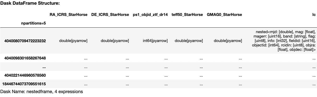
# join hips FGK object table to ZTF sources
lsdb_joined = object_table.join(
ztf_sources,
left_on="ps1_objid_ztf_dr14",
right_on="objectid",
suffixes=("", ""))
# get joined dataframe
joined_ddf = lsdb_joined._ddf
# map partitions of jointed dataframe
ddf = joined_ddf.map_partitions(
lambda df: convert_to_nested_frame(df, nested_columns=lc_columns),
meta=convert_to_nested_frame(joined_ddf._meta, nested_columns=lc_columns),
)
nested_ddf = NestedFrame.from_dask_dataframe(ddf)Initialize Nested Dataframe
Nested Pandas Workflow
target = 88291272191

# load target photometry
lc = nested_ddf.loc[target].compute().lc
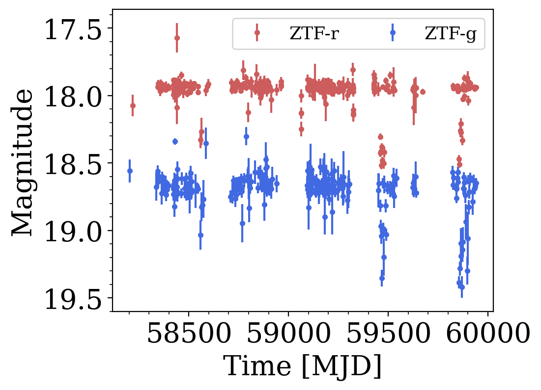
Nested Pandas Workflow
# Select only good Zubercal photometry
nested_ddf_update = nested_ddf.query("Teff > 5000")
nested_ddf_update = nested_ddf.query("lc.flag == 0 and lc.info == 0")

# Apply light curce quality check
q1 = nested_ddf_update.reduce(light_curve_quality,
                 "lc.mjd",
                 "lc.mag",
                 "lc.magerr",
                 "lc.flag",
                "lc.band",
                meta={"Nphot": np.float64})

# Update Nphot to the nested table and query
nested_ddf_update = nested_ddf_update.assign(Nphot=q1['Nphot'])
nested_ddf_update = nested_ddf_update.query("Nphot>100")

q2 = nested_ddf_update.reduce(evaluate_updated, # custom dipper finding pipeline
                         "lc.mjd",
                         "lc.mag",
                         "lc.magerr",
                         "lc.flag",
                         "lc.band",
                        meta={name: np.float64 for name in column_names}).to_parquet(f"{save_dir}")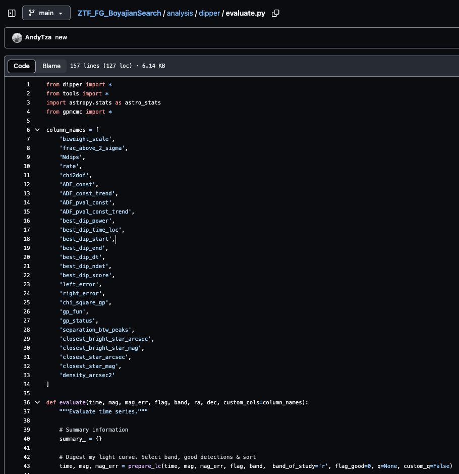
Custom Python time-series calculations/pipeline
Challenges
DASK memory management and sacalability for large and complex computations
How does LSDB sky partitioning affect Nested Pandas performance?
Resume DASK jobs after failure point
Documentation
(i.e more examples
of complex time-series
analysis workflows)
Conclusions
Special thanks to Neven Caplar, Doug Branton, Wilson Beebe, Andy Connolly, and the LINCC Frameworks team for making this project possible!
We are conducting the largest systematic search for main-sequence/Boyajian star analogs with ZTF and Gaia.
Both Large Survey DataBase (LSDB) and Neted Pandas, are pivotal tools for the success of this study - providing: data exploration, discovery, and rapid analysis
1.
2.
Project can be found on GitHub: github.com/dirac-institute/ZTF_FG_BoyajianSearch
Andy Tzanidakis// andytza.github.io // atzanida@uw.edu
2.
Our preliminary pipeline using LSDB + NP has already revealed over 80 new and exciting main-sequence dipper candidates!!
Backup Slides
Slow Dippers
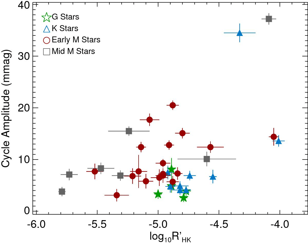
Typical activity cycles are in the 10-30 mmag
Mascareño + 2016
Slow and longterm secular trends can be found in simple light curve moments
ZTF Systematics
ZTF Systematics
ZTF DR17
Zubercal
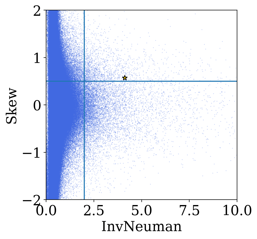
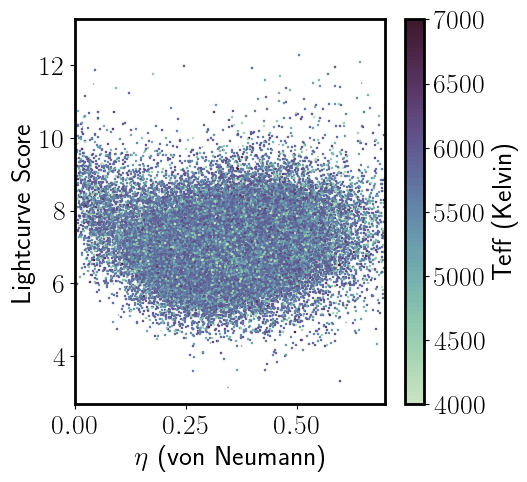
Light Curve Moments
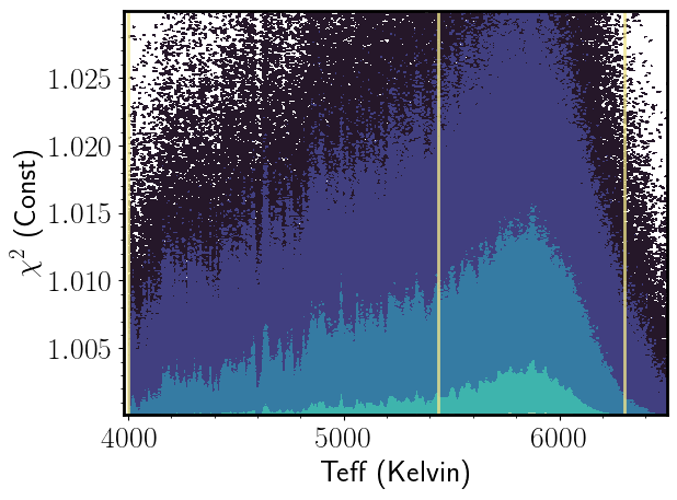
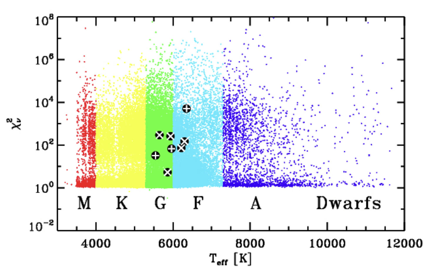
- Bimodal distribution in chi-square (assuming constant model) - some possible trends with Teff but biased sample...Overall good agreement with Ciardi et al. 2011
- Other trends in light curve moments, and possible classes/types of stellar variability... For example, bimodality in Von Neumann Ratio and light curve score, and other light curve moments...
Understanding & Collecting Auxiliary Data
Class I
Class II
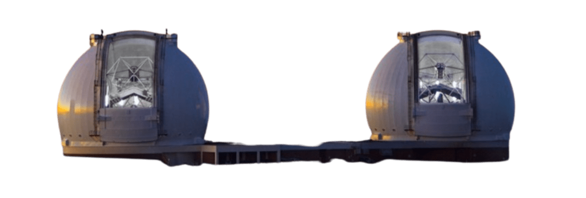
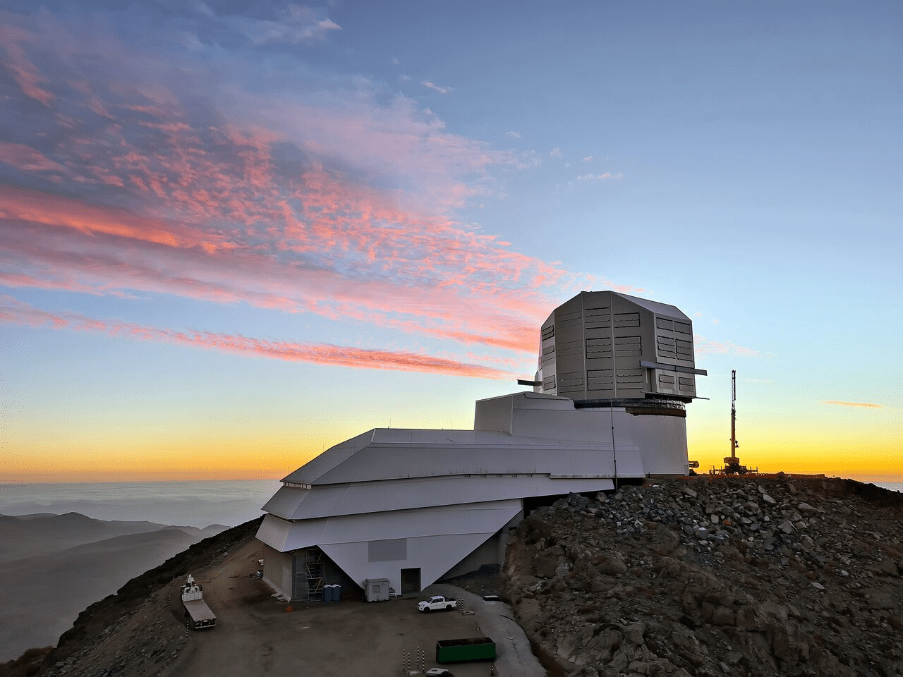
Vera C. Rubin Observatory
Legacy Survey of Space and Time (LSST)
Will resolve 17 billion stars!
🚨
~10M alerts per nigh!
- State-of-the-art techniques such as Temporal Convolutional Networks, by data augmenting known examples...
- Must carefully think about ToO programs targeting MS Dipper stars, since there will be numerous interesting candidates...!
- Careful follow-up programs on existing candidates
Backups

ZTF Systematics