Introduction to constrained registration trough diffeomorphic metric mapping.


Anton FRANÇOIS


Introduction
Point clouds & Landmarks
Images
Constrained
Metamorphosis
Modulated
Metamorphosis
Outline
Introduction
Shapes: Many Modalities
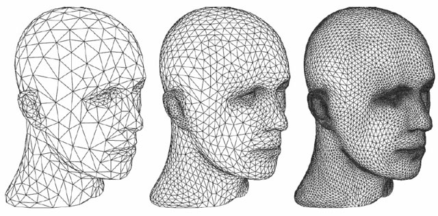
mesh
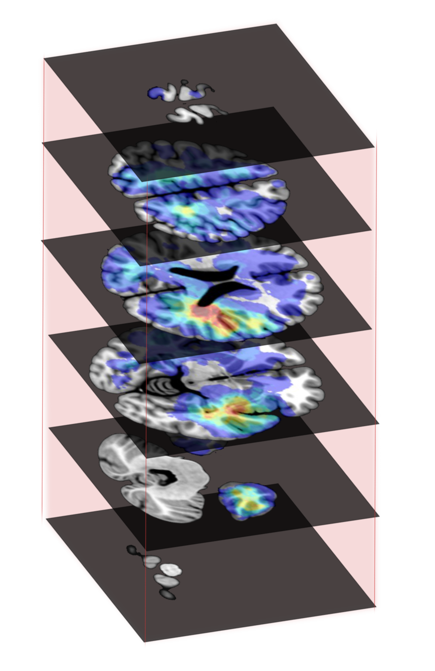
MRImages
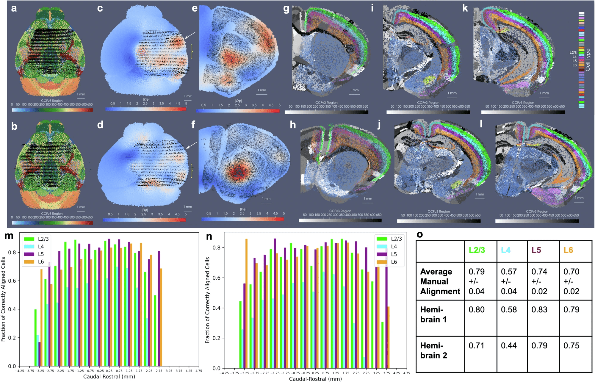
spatial transcriptomic
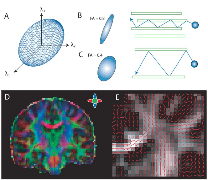
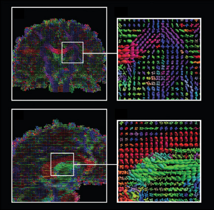
Diffusion Tensor Imaging (DTI)

Diffeomorphic image registration:
Finding a temporal smooth one-to-one
(non-linear) deformation to be biologically plausible (no holes, shearing, tearing...)
Image registration
Source
Target
Automatic non-linear
matching
LDDMM: Large Diffeomorphic Deformation Metric Mapping
With modern methods
J. Sassen, 2024
Recent examples
Recent examples
J. Sassen, 2024
Recent examples
J. Sassen, 2024
Recent examples
Shape Spaces

(Point clouds & Landmarks)
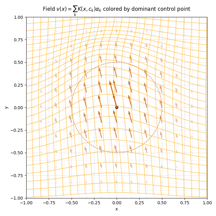
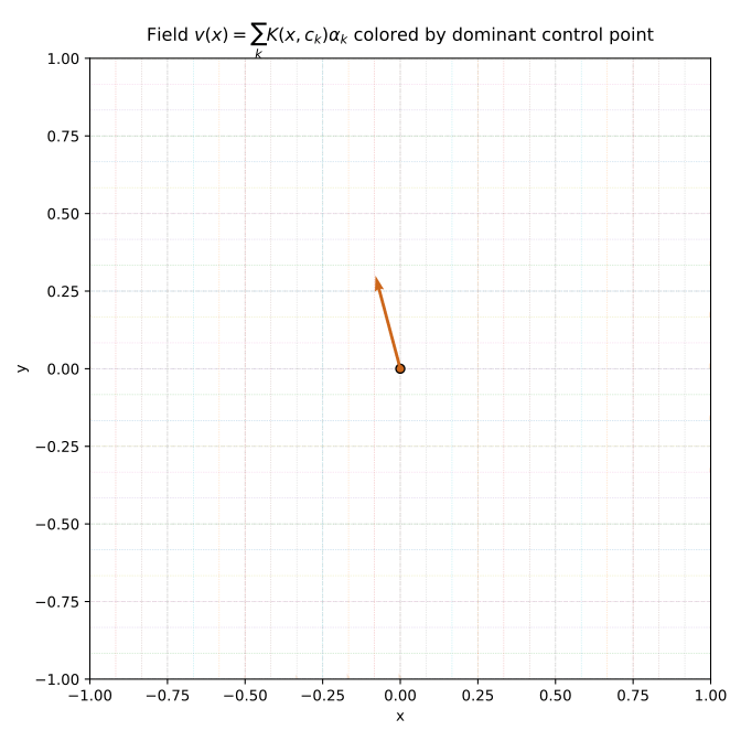
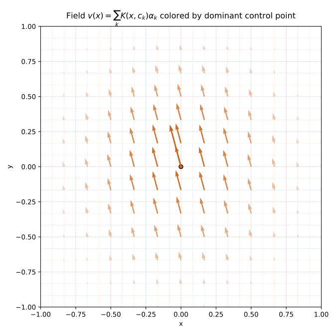
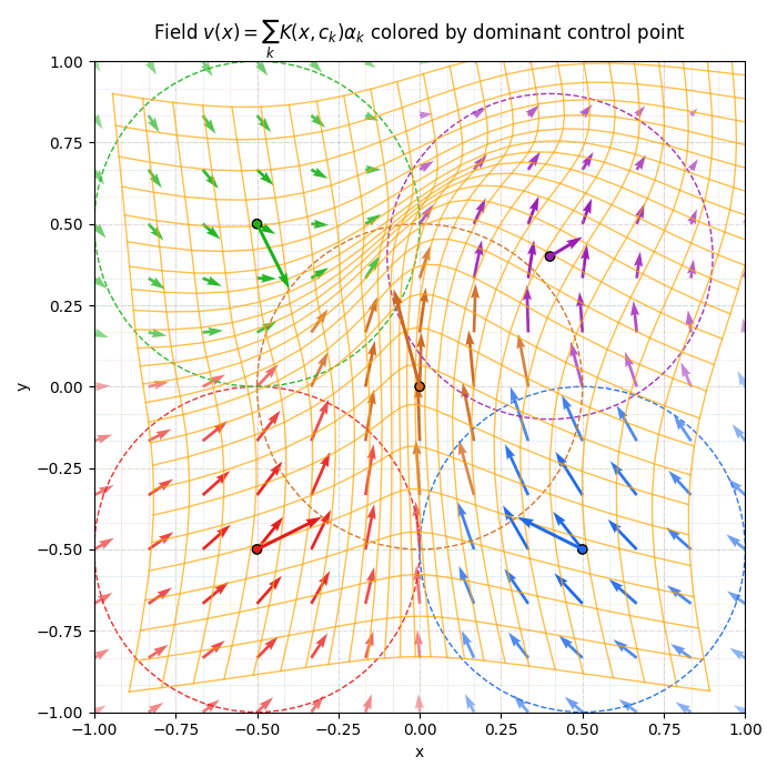
Ponctual support
- \(\Omega\) : space and \(x \in \Omega\)
- \( \{c_k\}_{k \in \llbracket 1, N\rrbracket } \) : control points
- \( \{\alpha_k\}_{k \in \llbracket 1, N\rrbracket } \) : momenta or vector weights, \(\forall k, \alpha_k \in \mathbb R ^d\)
- \(K \) : Radial basis function
- \(\Phi(x) = x + v(x)\) : Deformation
\[v(x) = \sum_{k=1}^N K(x, c_k)\alpha_k \]
\(c_1\)
\(\alpha_1\)
Deformation parametrized trough vector fields
Ensuring the diffeomorphism
To this end, we make the control points \(c_k\) and weights \(\alpha_k\) to depend on a “time” \(t \in [0,1]\) that plays the role of a variable of integration.
\[ v(t,x) = \sum_{k=1}^{N} K(x, c_k(t)) \alpha_k(t) \]
a particule \(x\) follows the integral curve according to the PDEs
\[\dot x(t) = \frac{dx_t}{dt} = v(t,x(t)), \qquad x(0) = x_0\]
\[\dot c(t) = K(c(t), c(t)) \alpha (t), \qquad c(0) = c_0 \]
the transformation is uniquely caracterized by the set of initials condition \(\{x_0, c_0, \alpha_0\}\).
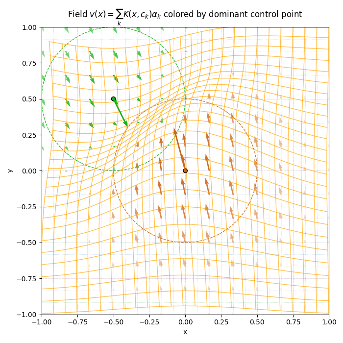
Norm on vectors fields
Given two vectors fields
\[v_1 = \sum_i K(\quad , c_i)\alpha_i;\qquad v_2 = \sum_j K(\quad, c_j') \beta_j \]
we define the scalar product
\[\langle v_1, v_2 \rangle_V = \sum_i \sum_j \alpha_i^\top K(c_i, c'_j) \beta_j \]
and the norm \(V\):
\[\|v\|_V^2 = \langle v, v \rangle_V \]
Let \(V\) be the Reproducing Kernel Hilbert Space (RKHS) of vector fields whose kernel is \(K\). We denote \(L: V \rightarrow V^*\) the Riesz operator such that \[\|v\|^2_V = ( Lv,v).\]
V is an admissible RKHS of vector fields.
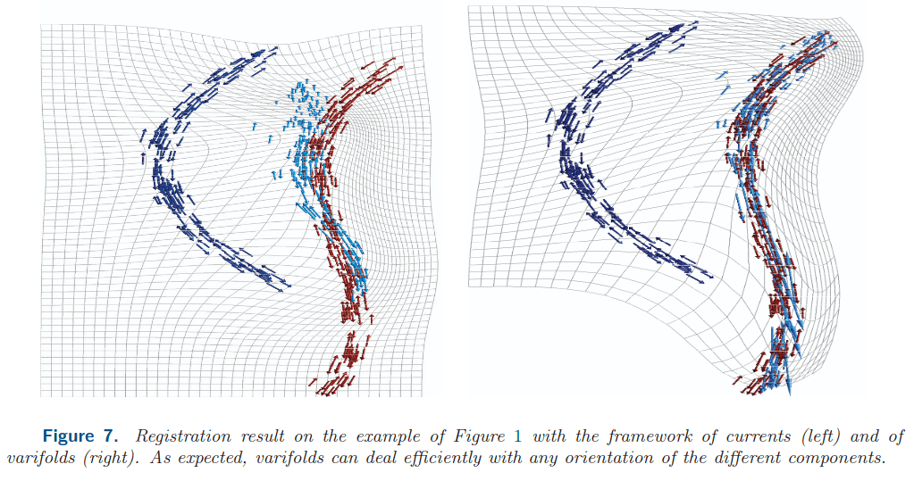
Varifold distance

\[\langle S, S' \rangle_{W^*} = \sum_i \sum_j K(c_i, c_j') \frac{(n_i ^\top n_j')^2}{|n_i| |n'_j|}\]
\[d_W(S, S') = \|S - S'\|_{W^*}^2 = \langle S, S \rangle_{W^*} + \langle S', S' \rangle_{W^*} - 2 \langle S, S' \rangle_{W^*}\]
Varifold distance
\[\langle S, S' \rangle_{W^*} = \sum_i \sum_j K(c_i, c_j') \frac{(n_i ^\top n_j')^2}{|n_i| |n'_j|}\]
\[d_W(S, S') = \|S - S'\|_{W^*}^2 = \langle S, S \rangle_{W^*} + \langle S', S' \rangle_{W^*} - 2 \langle S, S' \rangle_{W^*}\]
\(c_i\)
\(n_i\)

\(n_i\)
\(c_i\)
\[\langle S, S' \rangle_{W^*} = \sum_i \sum_j K(c_i, c_j') \frac{(n_i ^\top n_j')^2}{|n_i| |n'_j|}\]
\[d_W(S, S') = \|S - S'\|_{W^*}^2 = \langle S, S \rangle_{W^*} + \langle S', S' \rangle_{W^*} - 2 \langle S, S' \rangle_{W^*}\]
Varifold Norm
\(n_i\)
\(n_j'\)
\[\langle S, S' \rangle_{W^*} = \sum_i \sum_j K(c_i, c_j') \frac{(n_i ^\top n_j')^2}{|n_i| |n'_j|}\]
\[d_W(S, S') = \|S - S'\|_{W^*}^2 = \langle S, S \rangle_{W^*} + \langle S', S' \rangle_{W^*} - 2 \langle S, S' \rangle_{W^*}\]
Varifold Norm
Results
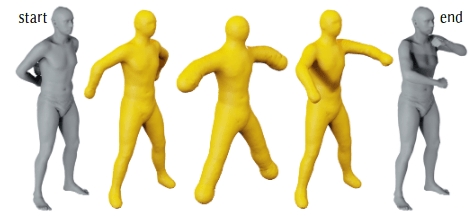
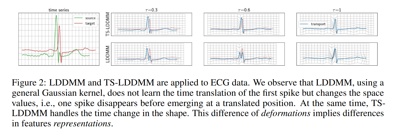
Time Series - LDDMM
Time Series - LDDMM
Time Series - LDDMM
Graph : \(G(s) := \{(t,s(t)) : t \in I\}\)
Solved the problem by choosing a well crafted kernel:
\[ K_G((t,x),(t',x')) = \left(\begin{matrix} c_0 K_{\mathrm{time}} & 0 \\ 0 & c_1K_{\mathrm{space}} \end{matrix}\right)\]
Intensity fields
(Images)
Lagrangian Formulation
$$x'(t) = v(t,x)$$
Lagrangian scheme
Not suitable for images
Eulerian scheme
\(I_{t+\delta_t} = I_t - \delta_t(v_t \times\nabla I_t)\)
Eulerian Formulation
$$\partial_t I(t,x) = - v(t,x) \cdot \nabla I(t,x)$$
Integration of the geodesics equations
Semi-Lagrangian scheme principle
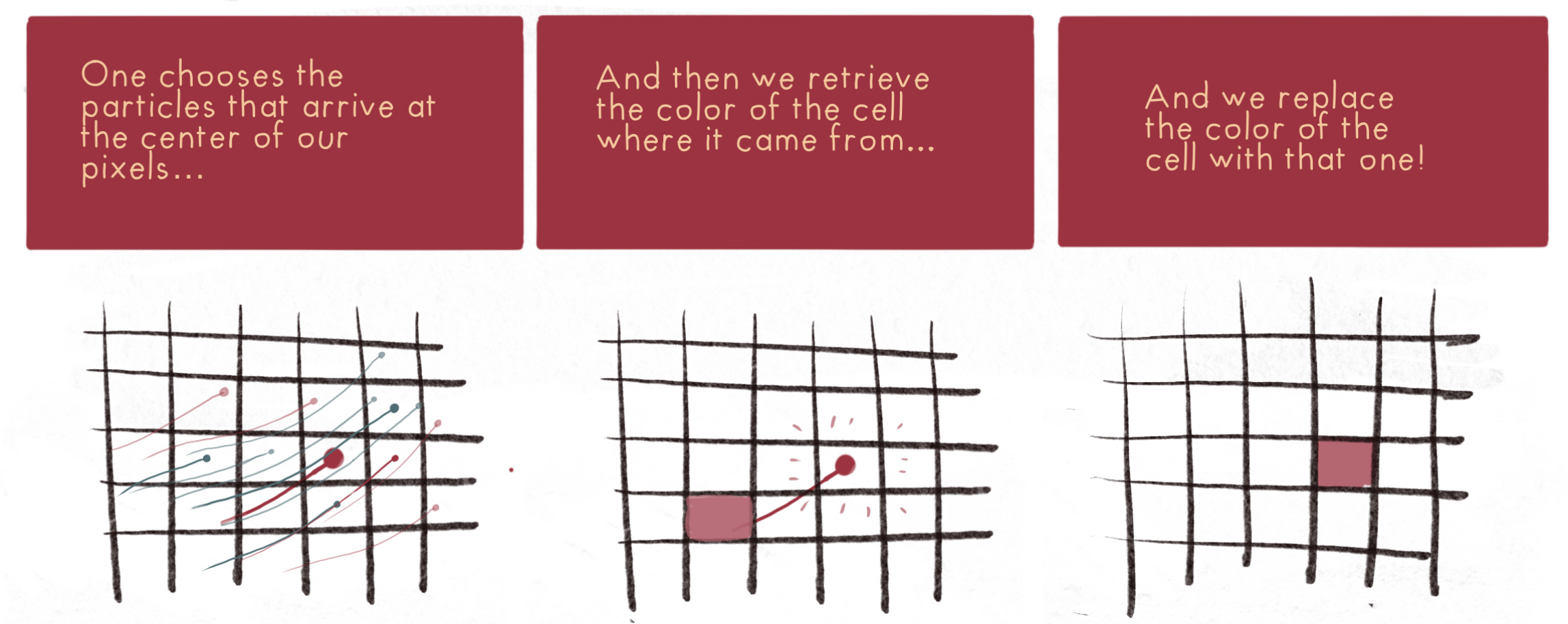
\(\partial_t I_t = v_t \cdot \nabla I_t\)
Semi-Lagrangian scheme
\(I_{t+\delta_t} = \mathrm{Interp}(I_t,\varphi^{v_t})\)

\(G\) is a group of diffeomorphisms
The deformation defined from the ordinary differential equation:
\[\partial_t \varphi_t = v_t \circ \varphi_t; \quad \varphi_0 = \mathrm{Id}\]
with \(v_t \in V,\forall t\in [0,1]\), is a diffeomorphism. We note \(\varphi^v \in G\) such a diffeomorphism.
\(G\) := Space of Deformations
Deformation as a flow of vector field

\[\partial_t \varphi_t = v_t \circ \varphi_t; \quad \varphi_0 = \mathrm{Id}\]
Image transport (advection): \[\partial_t I_t = v_t \cdot \nabla I_t \]
Deformed image
\(I_t = I_0 \circ (\varphi^v)^{-1}\)
The deformation acts on images.
Geodesic := Shortest path for the exact matching:
\[\mathrm{inf}_v \int_0^1 \|v_t\|_V^2 dt\]
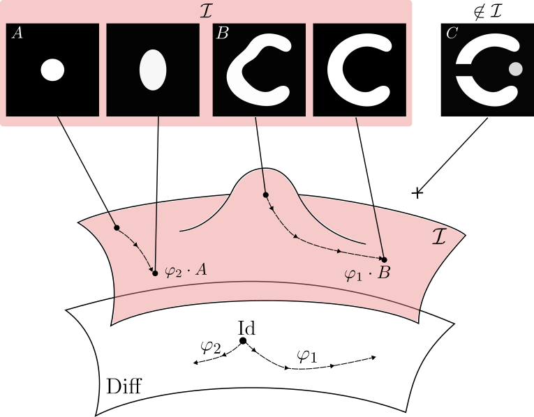
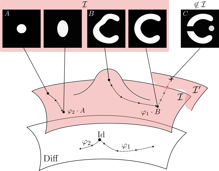
LDDMM can reach only images with same topology
Metamorphosis deforms images and adds intensity.
Making the registration of images B and C possible.
\[\partial_t I_t = v_t \cdot \nabla I_t\]
\[+ \mu z_t\]
Topology and appearances variations
Metamorphosis
\[\left\{\begin{array}{rl} v &= - \sqrt{ \rho } K_{V} (p \nabla I)\\ \dot{p} &= -\sqrt{ \rho } \nabla \cdot (pv) \\ z &= \sqrt{ 1 - \rho } p \\ \dot{I} &= - \sqrt{ \rho } v_{t} \cdot\nabla I_{t} + \sqrt{ 1-\rho } z.\end{array}\right. \]
Advection equation with sourceContinuity equation
Given the image evolution model
\[\dot I_t = - \sqrt{\rho}v_t \cdot \nabla I_t + \sqrt{1 - \rho} z_t; \qquad \rho \in [0,1]\]
and the Hamiltonian :
$$H(I,p,v,z) = - (p |\dot{ I}) - \frac{1}{2} \|v\|^2_{V} - \frac{1}{2}\|z\|^2_{2}. $$
we get the optimal trajectory as a geodesic of the form:
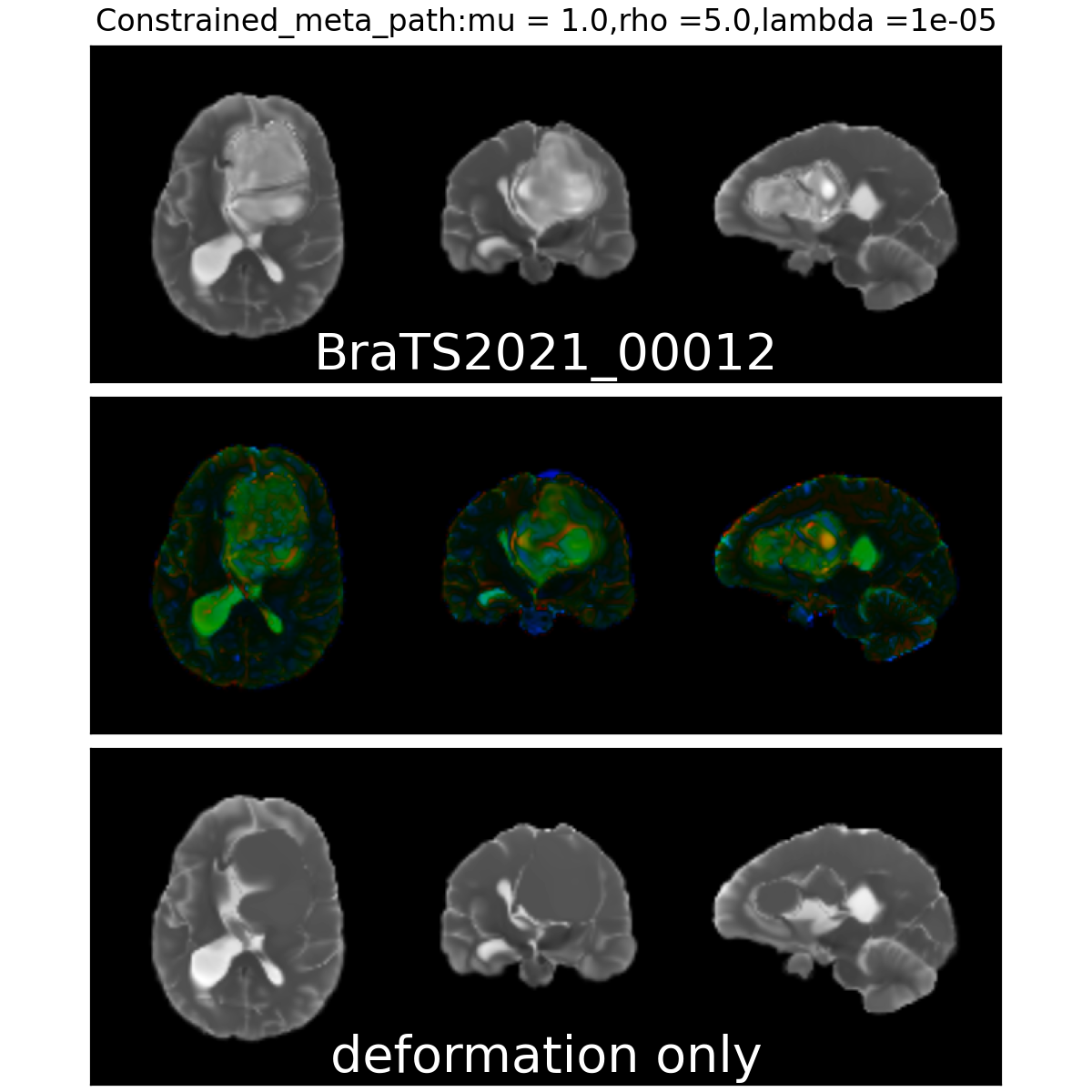
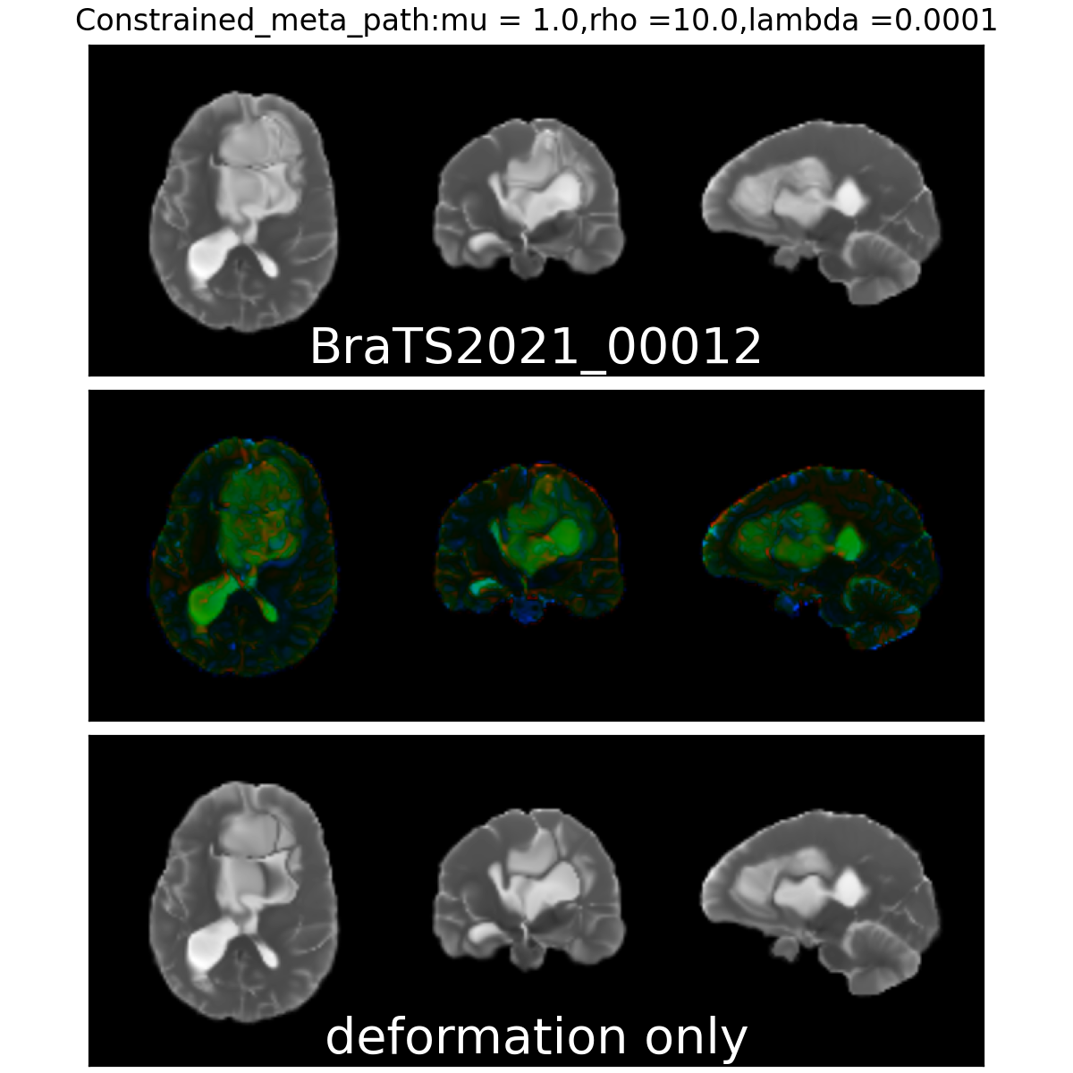
Constrained Metamorphosis
Registration with topological changes
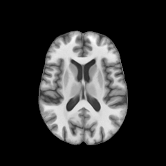
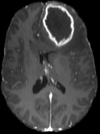
Healthy brain
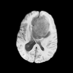
Brain with a glioblastoma
Anton François - 23/05/2023
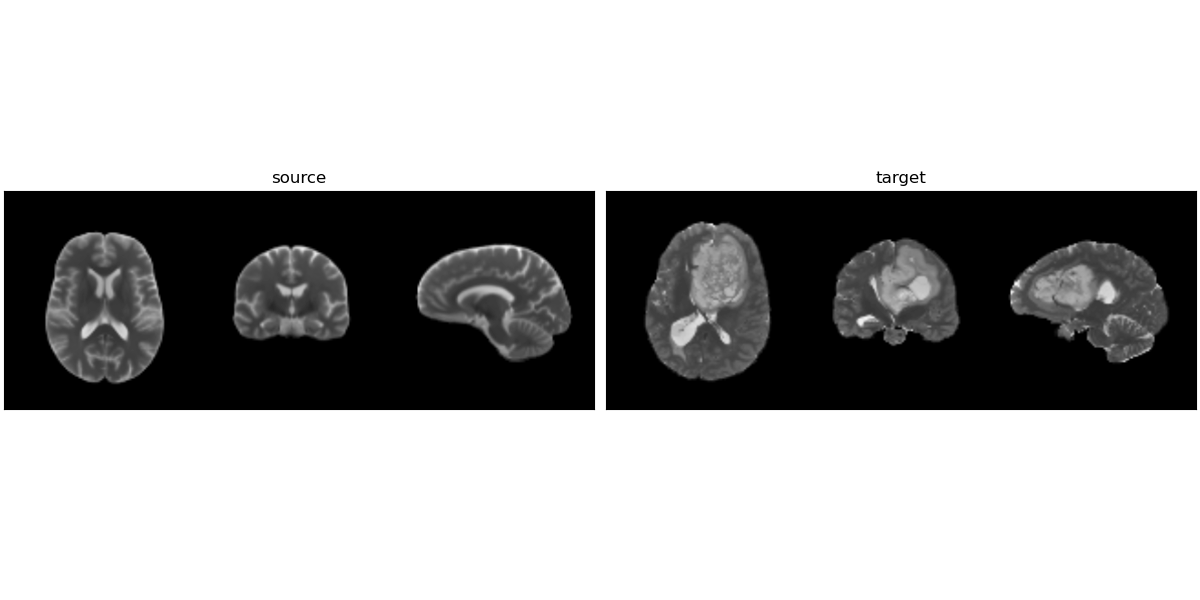
On real data: BraTS 2021
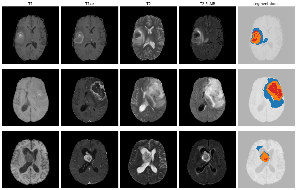
- Big data-set
- 4 modalities
- Glioblastoma ground truth segmentation
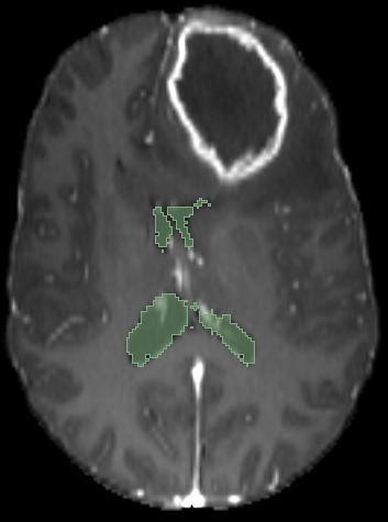
Registration validation using manually segmented ventricles (40 subjects).
Registered ventricles overlap measured with DICE score.
Constrained Metamorphosis
Let \((M_t)_{t\in [0,1]}\) and \((P_t)_{t\in [0,1]}\) be two continuous temporal masks and \(w_t \in V\), an admissible vector field.
By computing the Euler-Lagrange equation of the exact matching cost:
\[ E_{\mathrm{CM}}(I,v) = \int_0^1 \|v_t\|_V^2 + \rho \langle z_t, M_t z_t \rangle_{L^2} +\gamma\| P_t(v_t - w_t) \|_V^2 dt \]
and doing the variation with respect to \(I\) and \(v\) we obtain this set of geodesic equations:
Oriented & Weighted
\(s.t., I_0 = S, I_1 = T\)
Theorem:
$$\left\{\begin{array}{rl} v_t &= - \frac{\rho}{\mu (1 + \gamma P_t)} K \star (z_t\nabla I_t) + \frac{\gamma P_t }{1 + \gamma P_t} w_t\\ \dot z_t &= -\quad \nabla \cdot (z_t v_t) \\ \dot I_t &= - v_t \cdot\nabla I_t + \mu M_t z_t\end{array}\right.$$
\(\frac{\rho}{\mu(1+\gamma P_t)}\)
\(\frac{\gamma P_t}{1+\gamma P_t}\)
\(M_t\)
\(M_t\)
\(\|P_t(v_t - w_t) \|^2_V\)
Constrained Metamorphosis
Results on ToyExamples
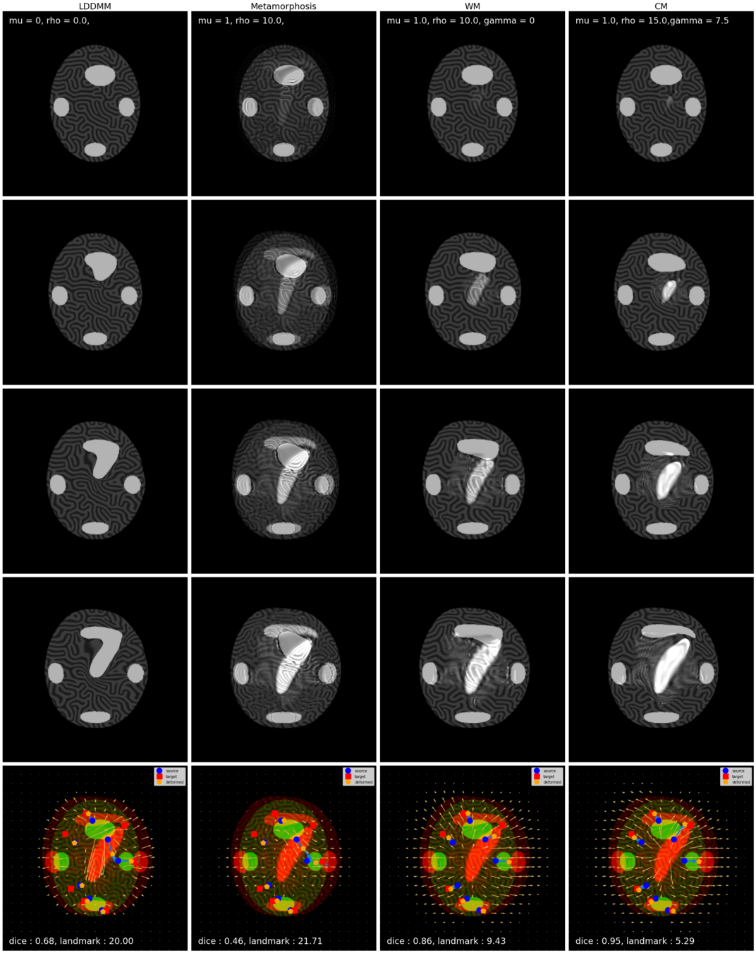
LDDMM
Classical Metamorphosis
source target
CM
WM
\(I_t\)
\(I_t\) & \(\varphi^{v_t}\)
\(z_t\)
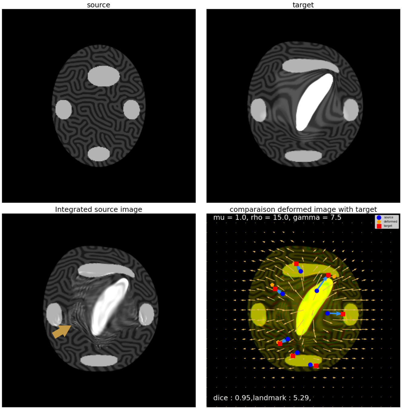
Constrained Metamorphosis
Results on ToyExamples
Constrained Metamorphosis
Weighted Metamorphosis
Qualitative results
Quantitative Results:
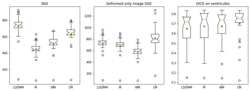
Lower the better
Higher the better
Modulated Metamorphosis
The standard \(n\)-Simplex is the subset of \(\mathbb R^{n+1}\) given by
$$\Delta^n = \left\{p \in \mathbb R^{n+1} : \forall i \in \{1,\cdots,n+1\}, p_i > 0; \sum_{i=1}^{n+1} p_i = 1\right\}.$$
A path on the 2-Simplex fig from [Jasminder, 2020]


Data from :
segmented MRI
Data Nature
Rigid alignment
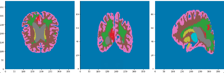
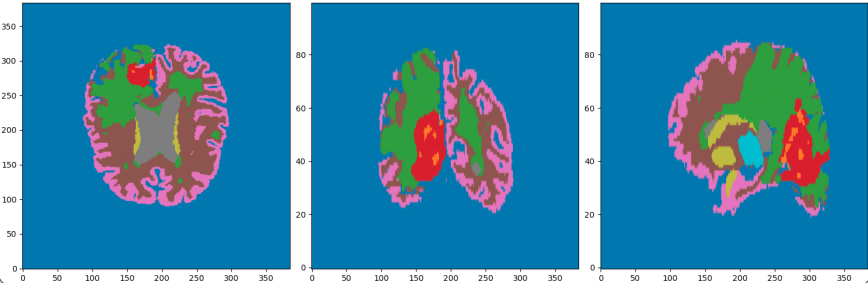
- Cancerous Growth (red - orange)
- White Matter Intensity reallocations (orange)
- Ventricule expansion (gray)
Registration difficulties
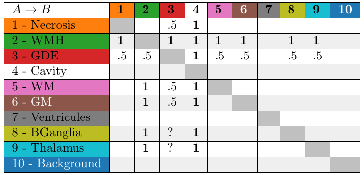
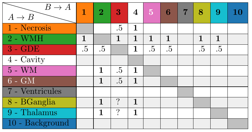
Control allocation matrix
Table with the values of \(\rho\) to transition from one class to another.
Up to now, the evolution of the image was described by:
\[\dot{q}_t = -\sqrt{1- \rho} \, v_t \cdot \nabla q_t + \sqrt{\rho} \, z_t., \rho \in \mathbb R\]
\(R =\)
\((\)
\()\)
Up to now, the evolution of the image was described by:
\[\dot{q}_t = -\sqrt{\rho} \, v_t \cdot \nabla q_t + \sqrt{1 - \rho} \, z_t., \rho \in \mathbb R\]
Let \( R \) be the control allocation matrix (CAM), such that each entry \( R(i,j) \) indicates the value of \( \rho \) for the transition from class \( i \) to class \( j \).
For \( f, g \in \Delta^d \), we define:
\[\rho(x, f, g) = \sum_{i \in \mathcal{C}} \sum_{j \in \mathcal{C}} f^i g^j R(i,j) = \left\langle f, gR \right\rangle.\]
We then introduce a new dynamics:
\[\dot{q}_t = -\sqrt{\tilde{\rho}_t} \, v_t \cdot \nabla q_t + \sqrt{1 - \tilde{\rho}_t} \, z_t,\]
where \( \tilde{\rho}_t = \rho(x, q_t, T) \).
Adapative re-allocation control
Conclusion


github.com/antonfrancois/Demeter_metamorphosis
- Tools to register without learning
- Introduce the data specificity to the model to really gets the expected result
- Join with a statistical model pour harness the best of both worlds. (Hopefully)
- The semi-Lagrangian scheme is more stable
- Open-Source Metamorphosis on the GPU, with autodiff.
- Made for prototyping
Anton François - 04/06/2024