Longitudinal MRI registration
Implementing metamorphoses on the simplex with a focus on GPU-memory optimisation


Anton FRANÇOIS
17 juin 2025
a work realised with Alain TROUVÉ

The RADIO-AIDE project investigates the neurotoxic mechanisms involved in the initiation and temporal progression of cognitive disorders following brain radiotherapy.
ANR:
Data on:

Preprocessed by:
Project overview
Talk outline
1. Demeter_Metamorphosis implementation - a focus on the GPU
2. Class dependent Weighted Metamorphosis
- Introduction to Metamorphosis
- Demeter structure
- GPU behaviour
- Checkpoints
- L-BFGS
- Model
- Data explanation
- Metamorphosis on the Simplex
- Selective strategy for deformation VS reallocation
- New model.
1. Demeter_Metamorphosis implementation - a focus on the GPU
2. Class dependent Weighted Metamorphosis
1.Demeter_Metamorphosis implementation
a focus on the GPU
1.1 Introduction to Metamorphosis
1.1 Introduction to Metamorphosis

LDDMM can reach only images with same topology
Metamorphosis deforms images and adds intensity.
Making the registration of images B and C possible.
\[\partial_t I_t = \sqrt{\rho}v_t \cdot \nabla I_t\]
\[+ \sqrt{1 - \rho} z_t\]
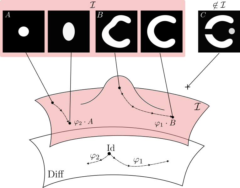
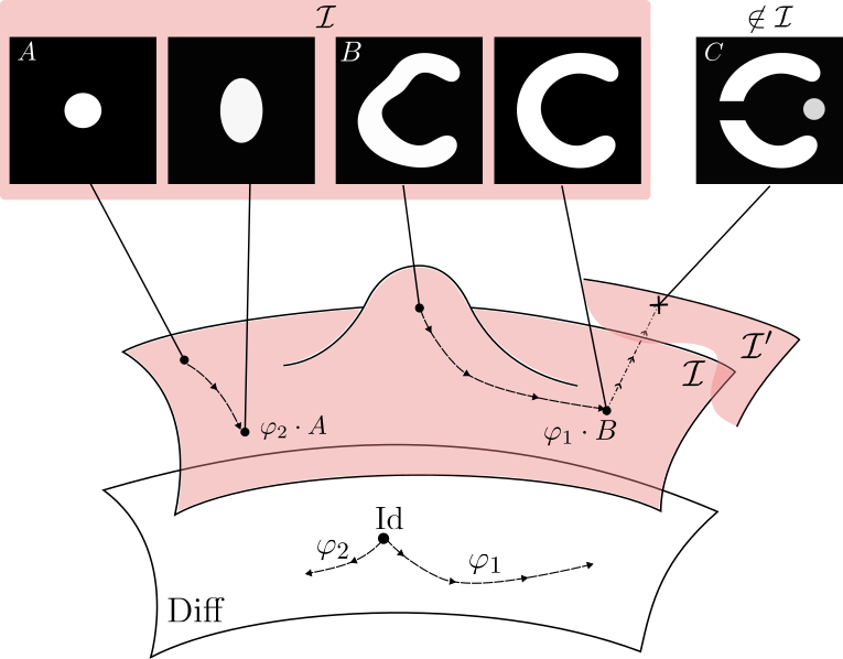
Topology and appearances variations
Anton François - 12/02/2025
A first Example
Metamorphosis

Source
Target
LDDMM
Anton François - 12/02/2025


Metamorphosis
A Metamorphosis on \(\mathcal I\) is a pair of curves \((\varphi_t, \psi_t)\), respectively on \(G\) and \(\mathcal I\), with \(\varphi_0 = \mathrm{Id}\).
\(G\) := Space of Deformations
\(\mathcal I\) := Space of images
\(\psi_t\) is the intensity changes evolution part: \(I_t = \psi_t \circ (\varphi_t)^{-1}\)
Anton François - 12/02/2025
Strategy overview
\(G\) := Space of Deformations
\(\mathcal I\) := Space of images
How to register in practice?
- Determine the geodesic expression by solving an exact-matching problem
- Relax the problem with inexact matching. Optimize through geodesic shooting.
Anton François - 12/02/2025
Exact matching formulation.
\[\left\{\begin{array}{rl} v &= - \sqrt{ \rho } K_{V} (p \nabla I)\\ \dot{p} &= -\sqrt{ \rho } \nabla \cdot (pv) \\ z &= \sqrt{ 1 - \rho } p \\ \dot{I} &= - \sqrt{ \rho } v_{t} \cdot\nabla I_{t} + \sqrt{ 1-\rho } z.\end{array}\right. \]
Advection equation with sourceContinuity equation
Given the image evolution model
\[\dot I_t = - \sqrt{\rho}v_t \cdot \nabla I_t + \sqrt{1 - \rho} z_t\]
and the Hamiltonian :
$$H(I,p,v,z) = - (p |\dot{ I}) - \frac{1}{2} \|v\|^2_{V} - \frac{1}{2}(z,z)_{2}. $$
we get the optimal trajectory as a geodesic of the form:
[Trouvé & Younes, 2005]
Anton François - 12/02/2025
1.2 Demeter structure
1.2 Demeter structure
We minimize this cost :
$$ H_\mathrm M (I,v) = \frac1 2 \left\| I_1 - T \right\|_2^2 + \frac \lambda 2\int_0^1 \|v_t\|_V^2 + \|z_t\|_{L_2}^2 dt $$
$$ \Leftrightarrow H_\mathrm M (p_0) = \frac1 2 \left\| I_1 - T \right\|_2^2 + \frac \lambda 2\left( \|p_0\nabla I_0\|_V^2 + \|z_0\|_{L_2}^2\right) $$
\(v_0 = - \sqrt \rho K\star (p_0 \nabla I_0) \)
\(\|v_0\|_V+ \|z_0\|_{L^2} = \|v_t\|_V + \|z_t\|_{L^2} ,\forall t\in [0,1]\)
Metamorphosis Optimisation
via Geodesic shooting
Anton François - 12/02/2025
\[\partial_t I_t = -\sqrt{\rho}v_t \cdot \nabla I_t\]
\[+ \sqrt{1 - \rho} z_t\]
Metamorphosis Optimisation
via Geodesic shooting
We minimize the inexact matching cost :
$$ H_\mathrm M (p_0) = \frac1 2 \left\| I_1 - T \right\|_2^2 + \frac \lambda 2\int_0^1 \|v_t\|_V^2 + \|z_t\|_{L_2}^2 dt $$
Geodesic Integration
\(p_0\)
\(I_1\)
Step 1:
Step 2:
We iterate over two steps:
\(\nabla H_M\) and adjoint equations computed
with auto differentiation.
Anton François - 12/02/2025
$$\left\{\begin{array}{rl} v &= - \sqrt{ \rho } K_{V} (p \nabla I)\\ \dot{p} &= -\sqrt{ \rho } \nabla \cdot (pv) \\ z &= \sqrt{ 1 - \rho } p \\ \dot{I} &= - \sqrt{ \rho } v_{t} \cdot\nabla I_{t} + \sqrt{ 1-\rho } z.\end{array}\right. $$
Shooting step
A shooting schematic
Geodesic Integration step
\(p_0\)
\(I_1\)
Anton François - 12/02/2025
Shooting step
Geodesic Integration step
Geodesic Integration step
Geodesic Integration step
1.3 GPU behaviour
1.3 GPU behaviour
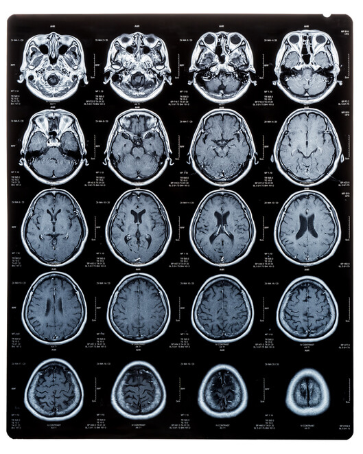
MR Images
Volumetric images
200x200x100 voxels
= 4e6 voxels.


1voxel take 32bytes (in float32)


1 image = 128e6 bytes = 122MB
The Data I'm looking at:
Image \(I\)
244 MB
128 MB
366 MB
732 MB
Momentum \(p\)
Residual \(z\)
Field \(v\)
A first guess about memory consumption
$$\left\{\begin{array}{rl} v &= - \sqrt{ \rho } K_{V} (p \nabla I)\\ \dot{p} &= -\sqrt{ \rho } \nabla \cdot (pv) \\ z &= \sqrt{ 1 - \rho } p \\ \dot{I} &= - \sqrt{ \rho } v_{t} \cdot\nabla I_{t} + \sqrt{ 1-\rho } z.\end{array}\right. $$
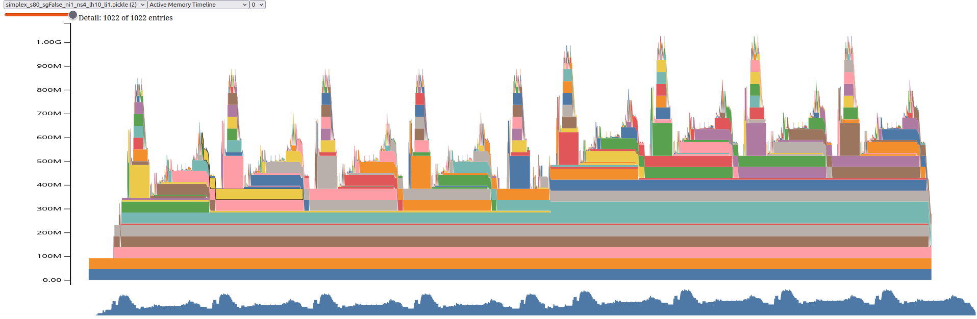
GPU utilisation
One integration step
$$\left\{\begin{array}{rl} v &= - \sqrt{ \rho } K_{V} (p \nabla I)\\ z &= \sqrt{ 1 - \rho } p \\ \dot{I} &= - \sqrt{ \rho } v_{t} \cdot\nabla I_{t} + \sqrt{ 1-\rho } z.\\ \dot{p} &= -\sqrt{ \rho } \nabla \cdot (pv) \end{array}\right. $$
Integration steps
Shooting forward
Image:
 80x80x100 pixels,
16e5 bytes,
48MB
x6 = 292MB
GPU utilisation
Full shooting, 4 steps
One shooting With Backward()
Image \(I\)
244 MB
128 MB
366 MB
732 MB
Momentum \(p\)
Residual \(z\)
Field \(v\)
7,15 GB
x 10 integration steps
Update prediction
1.4 Checkpoints
1.4 Checkpoints
torch.utils.checkpoint
Checkpoint a model or part of the model.
Activation checkpointing is a technique that trades compute for memory. Instead of keeping tensors needed for backward alive until they are used in gradient computation during backward, forward computation in checkpointed regions omits saving tensors for backward and recomputes them during the backward pass. Activation checkpointing can be applied to any part of a model.
In short, checkpointed code does not save the intermediary values in memory and must be recomputed.
Documentation
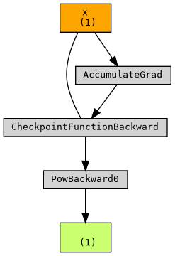
\(f(x) = (x^2 + \sin(x))^2\)
\(f(x) = g(x)^2\) with \(g(x) = x^2 + sin(x)\)
with an indermediary function
Minimal example
Let's assume that \( g \) is memory-intensive, and we create a checkpoint for it.
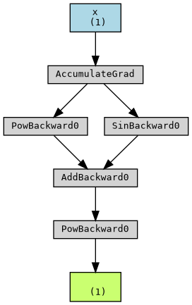
no checkpoint
with checkpoint
Geodesic Integration step
Shooting step
Geodesic Integration step
Geodesic Integration step
Geodesic Integration step
checkpoint
checkpoint integration step
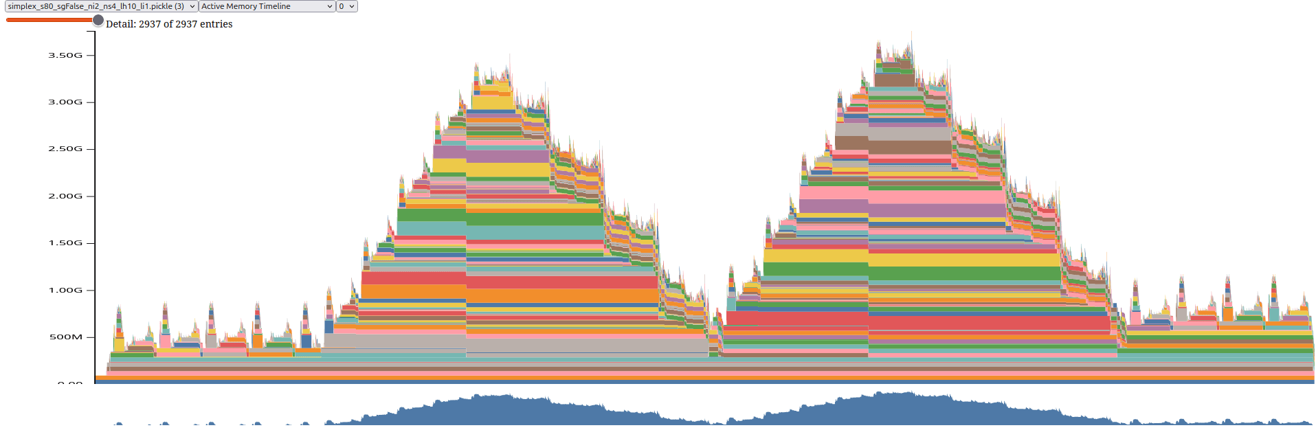
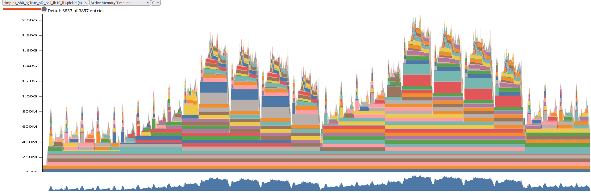
no checkpoint
checkpoint all
Checkpointing strategy
Result - Comparison
1.5 L-BFGS Optimisation
Rappel de cour
Torch implementation
class torch.optim.LBFGS()
Parameters (selection)
-
max_iter (int, optional) – maximal number of iterations per optimisation step (default: 20)
-
max_eval (int, optional) – maximal number of function evaluations per optimisation step (default: max_iter * 1.25).
-
history_size (int, optional) – update history size (default: 100). (But it is a lot more than needed)
-
line_search_fn (str, optional) – either ‘strong_wolfe’ or None (default: None). (But you should use 'strong_wolfe')
*(green text are my advise)
1.6 Modeling GPU utilisation
\(N\) := integration steps;
\(D\) := data size in bytes
\(M = \min(\text{lbfgs\_max\_iter} \times \text{n\_iter} , \text{lbfgs\_history\_size})\)
Parameter estimation:
Without checkpoint:
'a': 2.61022542, 'b': 39.20531525, 'c': 14595235.0, 'r2': 0.995706
with checkpoint:
'a': 3.06239906, 'b': 8.69422842, 'c': 23337559.0, 'r2': 0.921863
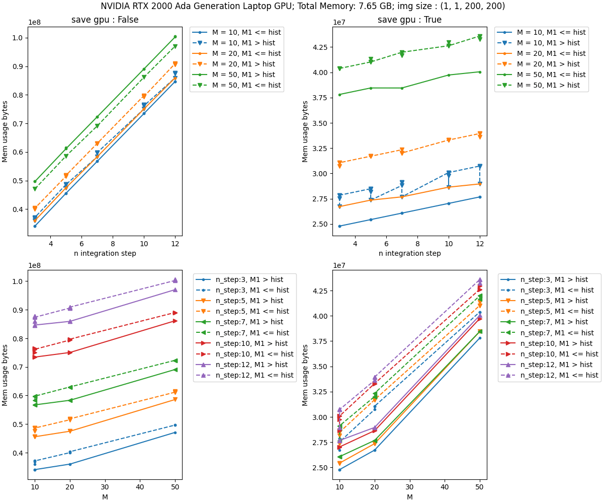
\(y = (a M + b N)\times D + c\).
Modeling GPU memory usage
Benchmark
lbfgs_history_size = 100
lbfgs_max_iter = 20
n_iter = 10
n_step = 10
lbfgs_history_size = 10
lbfgs_max_iter = 10
n_iter = 10
n_step = 10
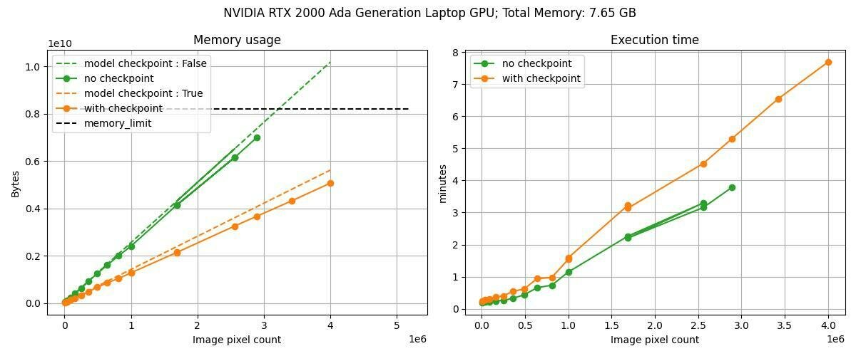
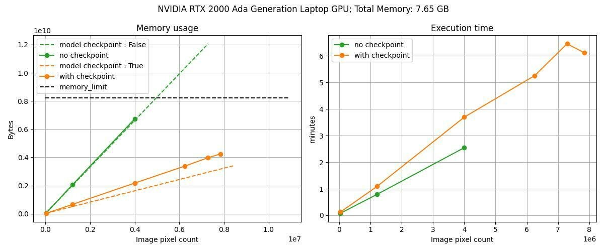
Conclusion
- Enabled the processing of higher resolution images
- Provided insights for users to adjust parameters without trial and error
- Enhanced the transparency of the code
2. Class Dependent Weighted Metamorphosis
2.1 A focus on the data

The standard \(n\)-Simplex is the subset of \(\mathbb R^{n+1}\) given by
$$\Delta^n = \left\{p \in \mathbb R^{n+1} : \forall i \in \{1,\cdots,n+1\}, p_i > 0; \sum_{i=1}^{n+1} p_i = 1\right\}.$$
A path on the 2-Simplex fig from [Jasminder, 2020]

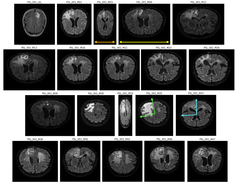
Data from :
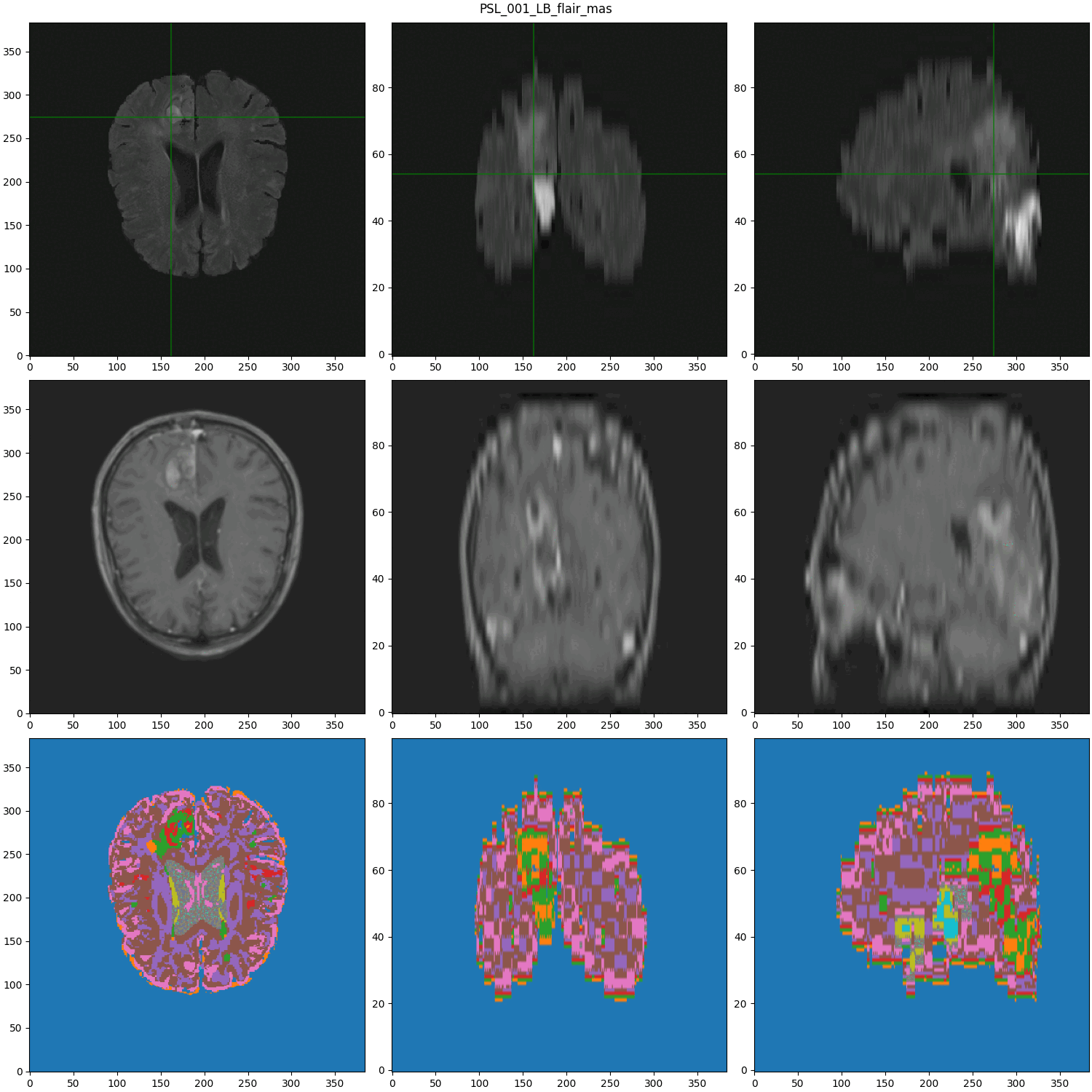
segmented MRI
Data Nature
Rigid alignment
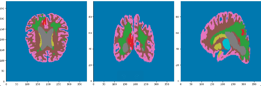
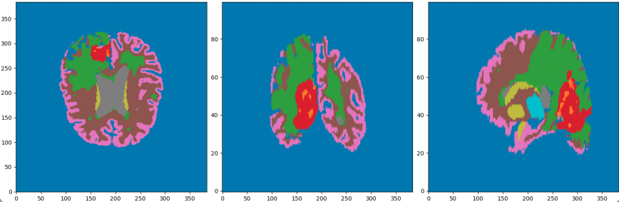
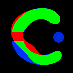
- Cancerous Growth (red - orange)
- White Matter Intensity reallocations (orange)
- Ventricule expansion (gray)
Registration difficulties
2.1 Metamorphosis on the simplex
2.1 Metamorphosis on the simplex
Let \(q\) be the "simplex image", (\(q(x) \in \Delta^n\)) and \(\tilde q : \Delta^n \mapsto S^n = \sqrt q\) the isometry from the simplex on the sphere. We set its evolution such that:
\[\partial_t\tilde q = -\sqrt{\rho} d \tilde q \cdot v + \sqrt{1 - \rho} z; \qquad\rho \in \mathbb R\]
$$\left\{\begin{array}{rl} \dot {\tilde q_t} &= - \sqrt{\rho} \nabla \tilde q_t \cdot v_t + \sqrt{1 -\rho} z_t\\ \dot p_t &= - \sqrt{\rho} \mathrm{div}(p_t \otimes v_t) - \sqrt{1 -\rho}<p_t, \tilde q_t>z_t\\ z_t &= \sqrt{1 - \rho} \Pi_{{\mathbb R}_{\tilde q}^\perp}(p)\\ v_t &= - \sqrt{\rho} K_V\left(\sum_{i=1}^{n+1} p_{t,i}\nabla \tilde q_{t,i} \right)\end{array}\right.$$
Metamorphosis on the Probability simplex
Together with the constraints \(\langle z, q \rangle = 0\) and the cost functional \(C(v, z) = \frac{1}{2} \|v\|_V^2 + \frac{1}{2} \|z\|_2^2,\) we recover the Hamiltonian \(H\) defined by
\[H(\tilde{q}, p, v, z) = \langle p, \partial_t \tilde{q} \rangle - \frac{1}{2} \|v\|_V^2 - \frac{1}{2} \|z\|_2^2.\] By computing the variations of \(H\) with respect to \(\tilde{q}, p, v,\) and \(z\), we recover the associated geodesic equations.
Metamorphosis on the Probability simplex
\(\rho = 1\) Pure Déformation
\(\rho = 0\) Ré-allocation
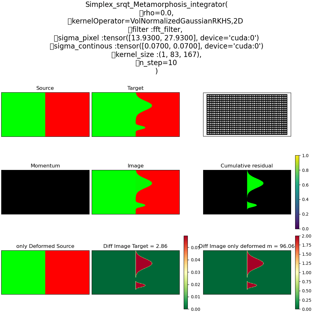
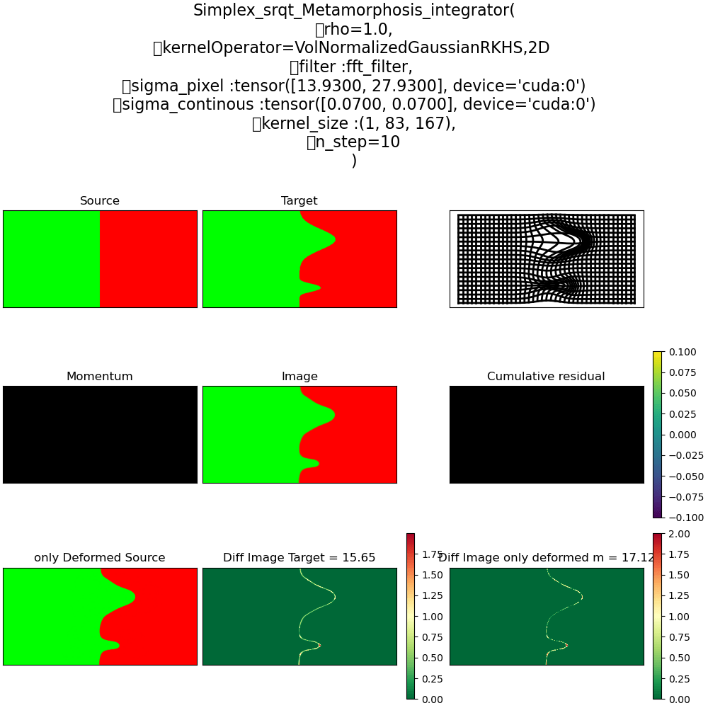
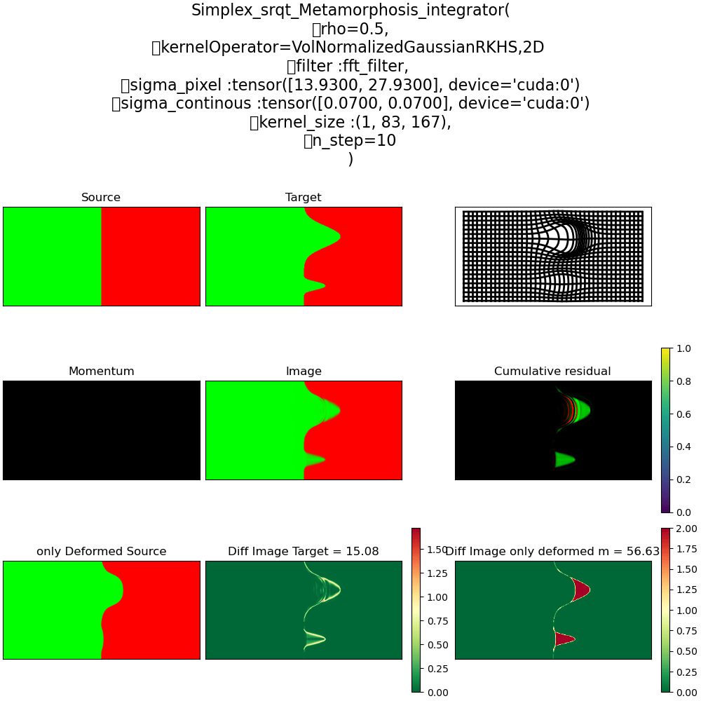
\(\rho = 0.5\) mix Déformation
2.2 Selective strategy for deformation VS Ré-allocations
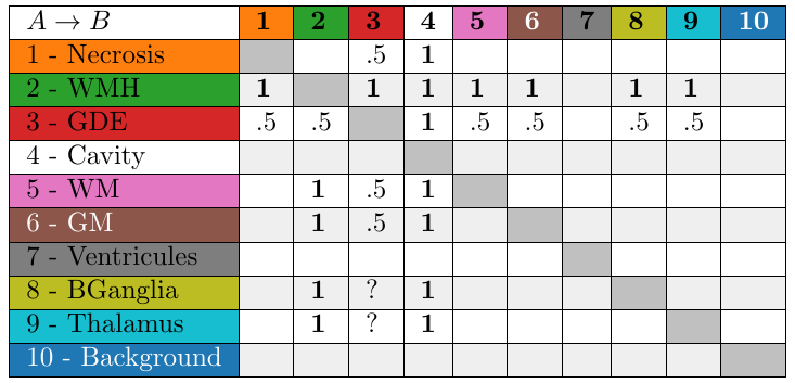
Control allocation matrix
Table with the values of \(\rho\) to transition from one class to another.
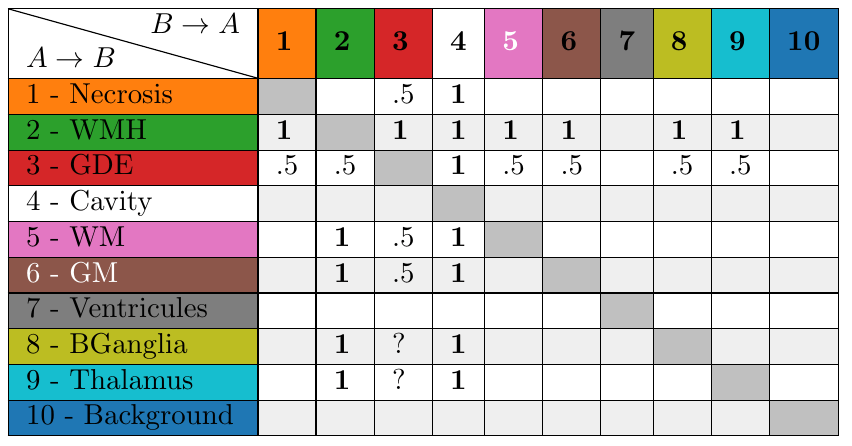
\(R =\)
\((\)
\()\)
Up to now, the evolution of the image was described by:
\[\dot{q}_t = -\sqrt{\rho} \, v_t \cdot \nabla q_t + \sqrt{1 - \rho} \, z_t., \rho \in \mathbb R\]
Let \( R \) be the control allocation matrix (CAM), such that each entry \( R(i,j) \) indicates the value of \( \rho \) for the transition from class \( i \) to class \( j \).
For \( f, g \in \Delta^d \), we define:
\[\rho(x, f, g) = \sum_{i \in \mathcal{C}} \sum_{j \in \mathcal{C}} f^i g^j R(i,j) = \left\langle f, gR \right\rangle.\]
We then introduce a new dynamics:
\[\dot{q}_t = -\sqrt{\tilde{\rho}_t} \, v_t \cdot \nabla q_t + \sqrt{1 - \tilde{\rho}_t} \, z_t,\]
where \( \tilde{\rho}_t = \rho(x, q_t, T) \).
Adapative re-allocation control
2.3 Class dependent
Weighted Metamorphosis
Our system dynamics are governed by
\[ \left\{ \begin{aligned} \dot{q}_t &= -\sqrt{\tilde{\rho}} \, dq_t \cdot v_t + \sqrt{1 - \tilde{\rho}} \, z_t, \\ \left\langle z_t, q_t \right\rangle &= 0, \\ C(v, z) &= \frac{1}{2} \left( \|v\|_V^2 + \|z\|^2 \right), \end{aligned} \right. \]
with
\[\tilde \rho = \rho(x, q, T) = \sum_{i \leq d} \sum_{j \leq d} q^i T^j R(i,j) = \left\langle q, RT \right\rangle.\]
we derive the Hamiltonian
\[ H(q,p,v,z,\lambda) = \left( p \mid -\sqrt{\tilde{\rho}} \, dq_t \cdot v_t + \sqrt{1 - \tilde{\rho}} \, z \right) - \frac{1}{2} \|v\|^2 - \frac{1}{2} \|z\|^2 - \lambda \left\langle z, q \right\rangle.\]
Hamiltonian
\[\left\{\begin{aligned}\lambda &= \frac{\left\langle \sqrt{1 - \tilde{\rho}} \, p, q \right\rangle}{\left\langle q, q \right\rangle} \\v &= -K_\sigma \ast \left( \sqrt{ \tilde{\rho} } \sum_{n=1}^{N+1} p_{n} \cdot \nabla q_{n} \right) \\z &= \sqrt{1 - \tilde{\rho}} \, p - \lambda q = \Pi_{\mathbb{R}_{q^\perp}}(\sqrt{1 - \tilde{\rho}} \, p) \\ \dot{q}_t &= -\sqrt{\tilde{\rho}} \, dq_t \cdot v_t + \sqrt{1 - \tilde{\rho}} \, z_t\\ \dot{p} &= - \mathbf{div}(\sqrt{\tilde{\rho}} pv^T)- \left\langle p,\frac{dq(v)}{2 \sqrt{\tilde{\rho}}}+ \frac{z}{2 \sqrt{1 - \tilde{\rho}}} \right\rangle RT - \lambda z\end{aligned}\right.\]
The geodesic equations associated to the Hamiltonian
\[ H(q,p,v,z,\lambda) = \left( p \mid -\sqrt{\tilde{\rho}} \, dq_t \cdot v_t + \sqrt{1 - \tilde{\rho}} \, z \right) - \frac{1}{2} \|v\|_V^2 - \frac{1}{2} \|z\|_2^2 - \lambda \left\langle z, q \right\rangle.\]
are
Geodesics
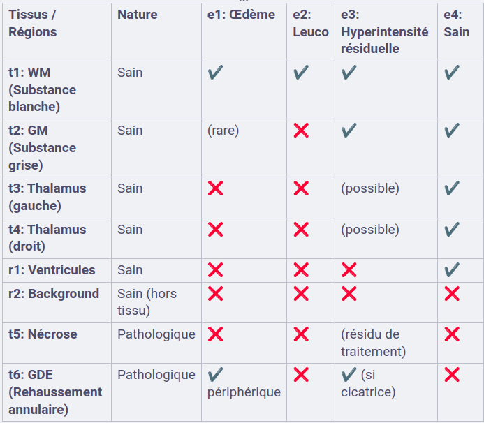
Régions
- WM (substance blanche)
- GM (Substance grise)
- Thalamus
- Ventricules
- Nécrose
- GDE (Rehaussement annulaire)
- Background
États
- Oedème
- Leucopathie
- autres Hyperintensité de T1ce
- Sain