Dr. Ashish Tendulkar
Machine Learning Techniques
IIT Madras
Models of Classification
Classification methods
- Discriminant functions learn direct mapping between feature vector \(\mathbf{x}\) and label \(y\).
-
Generative and discriminative models learn conditional probability distribution \(p(y|\mathbf{x})\) and assigns label based on that.
- Generative classifiers use Bayes theorem on class conditional densities \( p(\mathbf{x}|y)\) for features and prior probabilities of classes \(p(y)\).
- Discriminative classifiers use parametric models.
- Instance based models compare the test examples with the training examples and assign class labels based on certain measure of similarity.
Part I: Classification setup
Classification set up
- Predict class label \(y\) of an example based on the feature vector \(\mathbf{x}\).
- Class label \(y\) is a discrete quantity unlike a real number in regression set up.
Nature of class label
- Label is a discrete quantity - precisely an element in some finite set of class labels.
- Depending on the nature of the problem, we have one or more labels assigned to each example.
Types of classification
-
Single label classification - where each example has exactly one label.
- e.g. is the applicant eligible for loan?
- Label set: {yes, no}.
- Label either yes or no.
-
Multi-label classification - where each example has one or more labels.
-
e.g. identifying different types of fruits in a picture.
-
Label representation
- Single label classification: Label is a scalar quantity and is represented by \(y\).
- Multi-label classification: One or more labels hence vector representation \(\mathbf{y}\).
Label set: \(Y = \{y_1, y_2, \ldots, y_k\}\) has \(k\) elements/labels.
Depending on the presence of the label, the corresponding label is set to 1.
Example: Single label classification (Binary)
- Is the application eligible for loan?
-
Label set: \(\{yes, no\}\), usually converted to \(\{1, 0\}\)
- Label: either \(yes\ (1)\) or \(no (0)\).
- Training example:
- Feature vector: \(\mathbf{x}\) - features for loan application like age of applicant, income, number of dependents etc.
- Label: \(y\)
Example: Single label classification (Multiclass)
- Types of iris flower
- Label set: \(Y = \{versicolor, setosa, virginica\}\)
- Label: exactly one label from set \(Y\).
Example: Single label classification (Multiclass)
- Types of iris flower


versicolor
setosa
virginica
Image Source: Wikipedia.org
Label encoding in multiclass setup
Use one-hot encoding scheme for label encoding.
- Make use of a vector \(\mathbf{y}\) with components equal to the number of labels in the label set.
- In iris example, this would become:
Example: Label encoding (single label)
Let's assume that the flower has label versicolor, we will encode it as follows:
Note that the component of \(\mathbf{y}\) corresponding to the label versicolor is 1, every other component is 0.
Example: Multi-label Classification
- Label all fruits from an image.
- Label set: List of fruits e.g. \(\{apple,guava, mango, orange, banana, strawberry, \}\)
- Label: One or more fruits as they are present in the image.
Example: Multi-label Classification

Sample image
Image source: Wikipedia.org
Example: Multi-label Classification

Apple

Banana

Orange
Different fruits in the images are:
Example: Multi-label Classification
- Let's assume that the labels are \(\mathbf{apple}\), \(\mathbf{orange}\) and \(\mathbf{banana}\).
becomes
Training Data: Binary Classification
- Let's denote \(D\) as a set of \(n\) pairs of a features vector \(\mathbf{x}_{m \times 1}\) and a label \(y\), to represent examples.
- \(\mathbf{X}\) is a feature matrix corresponding to all the training examples and has shape \(n \times m\).
- In this matrix, each feature vector is transposed and represented as a row in this matrix.
Training Data: Binary Classification
Concretely, the feature vector for \(i\)-th training example \(\mathbf{x}^{(i)}\) can be obtained by \(\mathbf{X}[i]\):
Training Data: Binary Classification
- \(\mathbf{y}\) is a label vector of shape \(n \times 1\).
- The \(i\)-th entry in this vector gives label for \(i\)-th example, which is denoted by \(y^{(i)}\).
Training Data: Multi-class classification
\(D\): Set of \(n\) pairs of a feature vector \(\mathbf{x}\) and a label vector \(\mathbf{y}\) representing examples.
\(\mathbf{X}\) is an \(n \times m\) feature matrix.
\(\mathbf{Y}\) is a label matrix of shape \(n \times k\), where \(k\) is the total number of classes in label set.
Training Data: Multi-label classification
\(D\): Set of \(n\) pairs of a feature vector \(\mathbf{x}\) and a label vector \(\mathbf{y}\) representing examples.
\(\mathbf{X}\) is an \(n \times m\) feature matrix.
\(\mathbf{Y}\) is a label matrix of shape \(n \times k\), where \(k\) is the total number of classes in label set.
Multi-class and multi-label classification
- Multi-class classification: For \(\left(\mathbf{y}^{(i)}\right)^T\), exactly one entry corresponding to the class label is 1.
- Multi-label classification: For \(\left(\mathbf{y}^{(i)}\right)^T\), more than one entries corresponding to the class labels can be 1.
Differs in the content of label vector
Part II: Discriminant Functions
Discriminant functions learn direct mapping between feature vector \(\mathbf{x}\) and label \(y\).
\(\mathbf{x}\) Discriminant Function \(y\)
Model
In a binary classification set up with \(m\) features, the simplest discriminant function is very similar to the linear regression:
label
bias
weight vector
feature vector
Here label \(y\) is a discrete quantity unlike a real number in the linear regression set up.
Let's look at this discriminant function from geometric perspective.
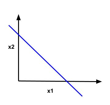
Geometric Interpretation
Geometrically, the simplest discriminant function, \(y = w_0 + \mathbf{w}^T \mathbf{x}\) represents a hyperplane in \(m-1\) dimensional space where \(m\) is the number of features.
| # features (m) | Discriminant function |
|---|---|
| 1 | Point |
| 2 | Line |
| 3 | Plane |
| 4 | Hyperplane in 3D space |
| ... | ... |
| m | Hyperplane in (m-1)-D space |
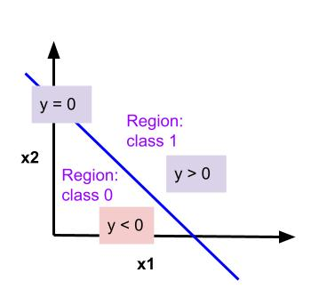
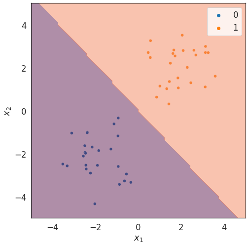
(m-1)-D hyperplane (which is line in this case) divides feature space into two regions one for each class:
- Region for class 1, where \(y > 0\)
- Region for class 2, where \(y < 0\)
The decision boundary between two classes is represented with (m-1)-D hyperplane: \(w_0 + \mathbf{w}^T\mathbf{x} = 0 \).
On decision boundary, \(y = 0\)
What does \(\mathbf{w}\) represent?
Consider two points \(\mathbf{x}^{(A)}\) and \(\mathbf{x}^{(B)}\) on the decision surface, we will have
Since \(y^{(A)} = y^{(B)} = 0\), \(y^{(A)} - y^{(B)}\) results into the following equation:
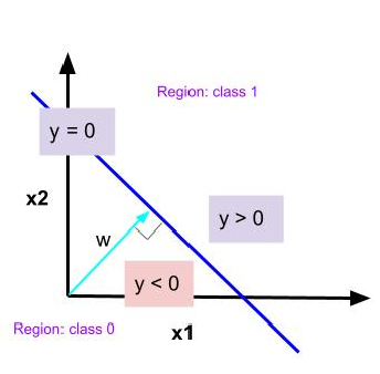
The vector \(\mathbf{w}\) is orthogonal to every vector lying within the decision surface, hence it determines the orientation of the decision surface.
What does \(w_0\) represent?
For points on decision surface, we have
Normalizing both sides with the length of the vector \(||\mathbf{w}||\), we get normal distance from the origin to the decision surface:
\(w_0\) determines the location of the decision surface
What does \(y\) represent?
\(y\) gives signed measure of perpendicular distance of the point \(\mathbf{x}\) from the decision surface.

Summary of geometric interpretation
- \(w_0\) determines the location of the decision surface.
- \(\mathbf{w}\) determines the orientation of the decision surface.
- \(y\) gives signed measure of perpendicular distance of the point \(\mathbf{x}\) from the decision surface.
- Decision surface divides feature space into two regions.
Now that we understand discriminant functions geometrically, let's explore how to classify an example \(\mathbf{x}\) with discriminant functions.
Inference
Discriminant function assigns label 1 to an example with feature vector \(\mathbf{x}\) if \((w_0 + \mathbf{w}^T\mathbf{x}) > 0 \) else assigns label 0.
Multiple classes
Assuming the number of classes to be \(k > 2\), we can build discriminant functions in two ways:
- One-vs-rest: Build \(k-1\) discriminant functions. Each discriminant function solves two class classification problem: class \(c_k\) vs \(not \ c_k\).
- One-vs-one: One discriminant function per pair of classes. Total functions = \({k \choose 2} = \frac{k (k-1)}{2}\)
Issues with one-vs-rest

- Each discriminant function separates \(C_k\) and not \(C_k\).
- Region of ambiguity is in green.
Issues with one-vs-one

- \(k(k-1)/2\) discriminant functions for each class pair \(C_i\) and \(C_j\).
- Each discriminant function separates \(C_i\) and \(C_j\).
- Each point is classified by majority vote.
- Region of ambiguity is in green.
How do we fix it?
A single \(k\)-class discriminant comprising \(k\) linear functions as follows:
Concretely:
Classification in \(k\)-discriminant functions
Assign label \(y_k\) to example \(\mathbf{x}\) if \(y_k > y_j, \forall j \ne k\)
The decision boundary between classes \(y_k\) and \(y_j\) corresponds to \(m-1\) dimensional hyperplane:
This has the same form as the decision boundary for the two class cases:
Now that we have a model of linear discriminant functions, we will study two approaches for learning the parameters of the model:
- Least squares
- Perceptron
Evaluation measures
- Confusion matrix
- Precision, recall, F1 scores, accuracy
- AUC of ROC and PR curves
Least square classification
Least square classification adapts linear regression for classification.
We use least square error as a loss function.
Least square error
The error at \(i\)-th training point is calculated as follows:
The total loss is the sum of square of errors between actual and predicted labels at each training point.
Note that the loss is dependent on the value of \(\mathbf{w}\) - as these value changes, we get a new model, which will result in different prediction and hence affects the error at each training point.
Optimization
Normal equation
Calculate derivative of loss function \(J(\mathbf{w})\) w.r.t. weight vector \(\mathbf{w}\). [refer to linear regression material for detailed derivation]
Set \(\dfrac{\partial J(\mathbf{w})}{\partial \mathbf{w}}\) to 0 and solve for \(\mathbf{w}\):
Whenever \(\mathbf{X}^T \mathbf{X}\) is not full rank, we calculate pseudo-inverse: \(\left( \mathbf{X}^T \mathbf{X} \right)^{-1} \mathbf{X}^T\)
Gradient Descent
We derive weight update rule in vectorized format as follows:
We will implement this update rule in gradient descent algorithm in colab.
Implementation from scratch and demo
def predict(X, w):
  z = X @ w
  return np.array([1 if z_val >= 0 else 0 for z_val in z])
def fit(X, y):
return np.linalg.pinv(X) @ yInference
Optimization through normal equation
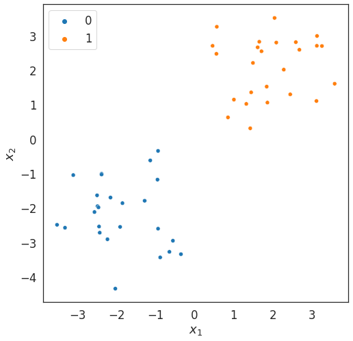
Training data
Decision boundary via LSC