Bayesian Deep Learning
Basics
Probability Theory and Bayesian Approach
Why go Bayesian?
- There's always some uncertainty
- Complex partially observed world
- Few observations
- Probability Theory is a great tool to reason about uncertainty
- Bayesians quantify subjective uncertainty
- Frequentists quantify inherent randomness in the long run
- People seem to interpret probability as beliefs and hence are Bayesians
The Bayesian Workflow
We want to make predictions about some \( x \)
- We formulate our prior beliefs about how the \( x \) might be generated
- We collect some data of already generated \( x \): $$ \mathcal{D}_\text{train} = (x_1, ..., x_N) $$
- We update our beliefs regarding what kind of data exist by incorporating collected data
- We now can make predictions about unseen data
- And collect some more data to improve our beliefs
Probability Theory 101
- We'll assume random variables have and are described by their densities
- \(X\) – random variable
- \(p(X=x)\) (\(p(x)\) for short) – its probability density function
- \(\text{Pr}[X \in A] = \int_{A} p(X=x) dx\) – distribution function
- In general several random variables \(X_1, ..., X_N\) have joint density $$ p(X_1=x_1, ..., X_N=x_n) $$
- It describes joint probability $$\text{Pr}(X_1 \in A_1, ..., X_N \in A_N) = \int_{A_1} ... \int_{A_N} p(x_1, ..., x_N) dx_N ... dx_1 $$
- If (and only if) random variables are independent, the joint density is just a product of individual densities
- Vector random variables are just a bunch of scalar random variables
- For 2 and more random variables you should be considering their joint distribution
Probability Theory 101
- \(\mathbb{E}_{p(x)} X = \int x p(x) dx\) – expected value
- \( \mathbb{E} [\alpha X + \beta Y] = \alpha \mathbb{E} X + \beta \mathbb{E} Y \)
- Law of the Unconscious Statistician $$ \mathbb{E} f(x) = \int f(x) p(x) dx $$
- \( \mathbb{V} X = \mathbb{E} [X^2] - (\mathbb{E} X)^2 = \mathbb{E}(X - \mathbb{E} X)^2 \) – variance
- If \(X\) and \(Y\) are independent, \( \mathbb{V}[\alpha X + \beta Y] = \alpha^2 \mathbb{V} X + \beta^2 \mathbb{V} Y \)
-
\( \text{Cov}(X, Y) = \mathbb{E} [X Y] - \mathbb{E} X \mathbb{E} Y \) – covariance
- \( \mathbb{V} [\alpha X + \beta Y] = \alpha^2 \mathbb{V}[X] + \beta^2 \mathbb{V}[Y] + 2 \alpha \beta \text{Cov}(X, Y) \)
- \(q_\alpha\) is called an \(\alpha\)-quantile of \(X\) if \(\text{Pr}[X < q_\alpha] = \alpha\) (equivalently \(\text{Pr}[X \ge q_\alpha] = 1 - \alpha\))
- In particular, \(q_{1/2}\) is called the median
ExampleS
- \(X\) is said to be Uniformly distributed over \((a, b)\) (denoted \(X \sim U(a, b)\) if its probability density function is $$ p(x) = \begin{cases} \tfrac{1}{b-a}, & a < x < b \\ 0, &\text{otherwise} \end{cases} \quad\quad \mathbb{E} U = \frac{a+b}{2} \quad\quad \mathbb{V} U = \frac{(b-a)^2}{12} $$
- \(X\) is called a Multivariate Gaussian (Normal) random vector with mean \(\mu \in \mathbb{R}^n\) and positive-definite covariance matrix \(\Sigma \in \mathbb{R}^{n \times n}\) (denoted \(x \sim \mathcal{N}(\mu, \Sigma)\)) if its joint probability density function is $$ \quad\quad\quad\quad\quad\quad\quad\quad\quad \quad \quad p(x) = \frac{1}{\sqrt{\text{det}(2 \pi \Sigma)}} \exp \left( -\tfrac{1}{2} (x-\mu)^T \Sigma^{-1} (x-\mu) \right) $$

$$ \mathbb{E} X = \mu $$
$$ \text{Cov}(X_i, X_j) = \Sigma_{ij} $$
More ExampleS
- \(X\) is said to be Categorically distributed with probabilities (non-negative and sum to 1) \(\pi_1, ..., \pi_K\) (denoted \(X \sim \text{Cat}(\pi_1, ..., \pi_K)\)) if its probability
densitymass function is
- \(X\) is called a Bernoulli random variable with probability (of success) \(p \in [0, 1]\) (denoted \(X \sim \text{Bern}(\pi)\)) if its probability mass function is $$ p(X = 1) = \pi \Leftrightarrow p(x) = \pi^{x} (1-\pi)^{1-x} $$ (yes, this is a special case of the categorical distribution)
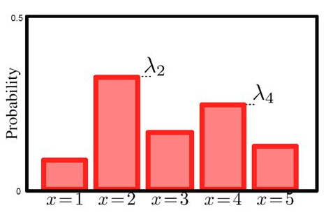
$$ p(X = k) = \pi_k \Leftrightarrow p(x) = \prod_{k=1}^K \pi_k^{[x = k]} $$
Probability Theory 101
- Joint density on \(x\) and \(y\) defines the marginal density on each of them: $$ p(x) = \int p(x, y) dy \quad\quad p(y) = \int p(x,y) dx $$
- Knowing value of \(y\) can reduce uncertainty about \(x\), expressed via the conditional density $$ p(X=x|Y=y) = \frac{p(x, y)}{p(x)} = \frac{p(X=x, Y=y)}{\int p(X=x, Y=z) dz} $$
- Thus $$ p(x, y) = p(y|x) p(x) = p(x|y) p(y) $$
- In general the chain rule is $$ p(x_1, \dots, x_N) = p(x_1) p(x_2 | x_1) p(x_3 | x_1, x_2) ... p(x_N | x_1, ..., x_{N-1}) $$
Example
- Suppose we're having two jointly Gaussian random variables \(X\) and \(Y\): $$(X, Y) \sim \mathcal{N}\left(\left[\begin{array}{c}\mu_x \\ \mu_y \end{array} \right], \left[\begin{array}{cc}\sigma^2_x & \rho_{xy} \\ \rho_{xy} & \sigma^2_y\end{array}\right]\right)$$
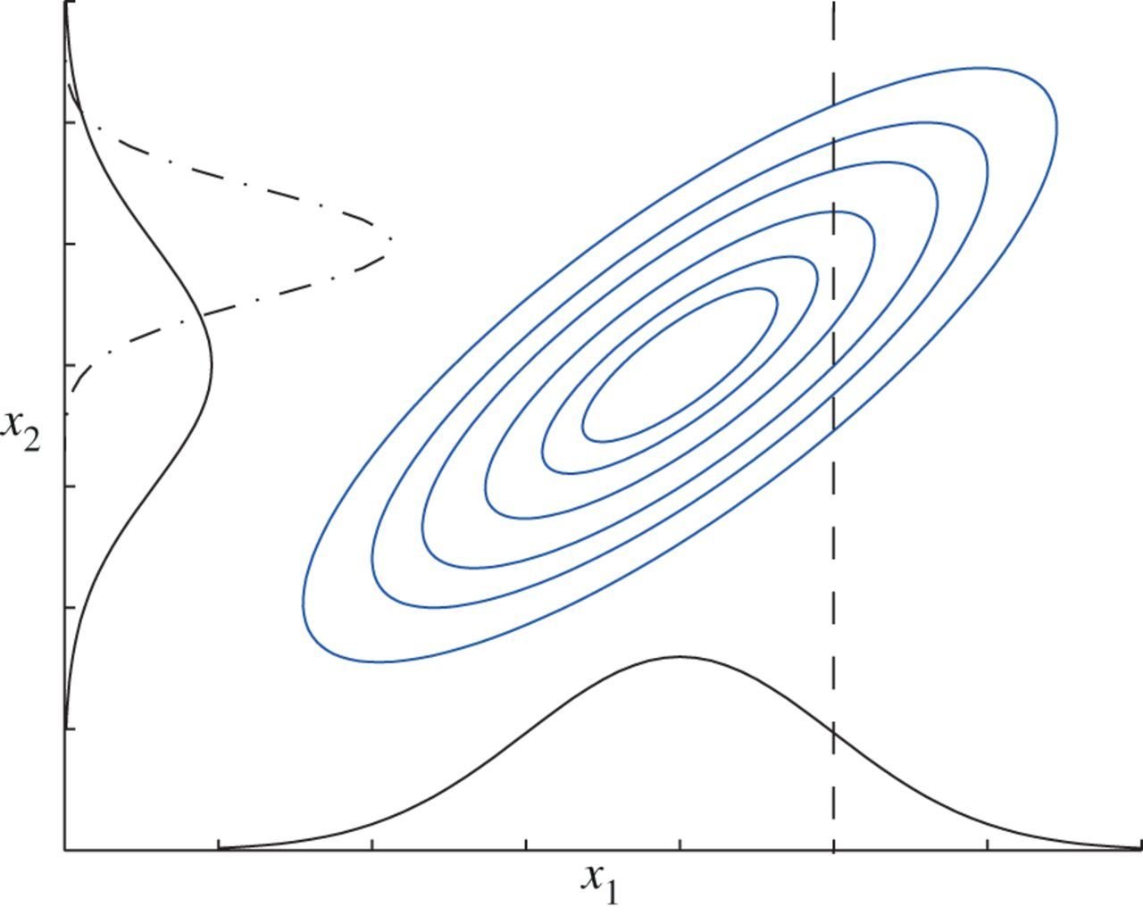
- Then one can show that marginal and conditionals are also Gaussian $$ p(x) = \mathcal{N}(x \mid \mu_x, \sigma^2_x) $$ $$ p(y) = \mathcal{N}(y \mid \mu_y, \sigma^2_y) $$ $$p(x|y) = \mathcal{N}\left(x \mid \mu_x + \tfrac{\rho}{\sigma_x^2} (y - \mu_y), \sigma^2_x - \tfrac{\rho_{xy}^2}{\sigma_y^2}\right)$$
Probability Theory 101
- This leads to the Bayes' theorem relating conditional distributions $$ p(y|x)= \frac{p(x, y)}{p(x)} = \frac{p(x|y) p(y)}{p(x)} $$
- If we're interested in \(y\), then these distributions are called
- \( p(x|y) \) – likelihood function
- \( p(y) \) – prior distribution
- \( p(y|x) \) – posterior distribution
- \( p(x) \) – model evidence or marginal likelihood
Bayesian Machine Learning 101
- We assume some data-generating model $$p(y, \theta \mid x) = p(y \mid x, \theta) p(\theta) $$
- \(x\) and \(y\) are observed
- \(\theta\) is not observed, called latent variable
- We obtain some observations \( \mathcal{D} = \{(x_n, y_n)\}_{n=1}^N \)
- We seek to make make predictions regarding \(y\) for previously unseen \(x\) having observed the training set \(\mathcal{D}\). Its uncertainty quantified by the posterior predictive distribution $$p(y \mid x, \mathcal{D}) = \int p(y \mid x, \theta) p(\theta \mid \mathcal{D}) d\theta $$
- This requires us to know the posterior distribution on model parameters \(p(\theta \mid \mathcal{D})\) which we obtain using the Bayes' rule
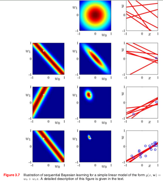
Example: Bayesian Linear Regression
- Suppose the model \(y \sim \mathcal{N}(\theta^T x, \sigma^2)\), with \( \theta \sim \mathcal{N}(\mu_0, \sigma_0^2 I) \)
- Suppose we observed some data from this model \( \mathcal{D} = \{(x_n, y_n)\}_{n=1}^N \) (generated using the same \( \theta^* \))
- We don't know the optimal \(\theta\), but the more data we observe – the more certain we are about possible values of \(\theta\) $$ p(\theta | \mathcal{D}) = \frac{\prod_{n=1}^N p(y_n| x_n, \theta) p(\theta)}{p(\mathcal{D})} = \mathcal{N}(\theta \mid \mu_N, \Sigma_N) $$
- Posterior predictive would also be Gaussian $$ p(y|x, \mathcal{D}) = \mathcal{N}(y \mid \mu_N^T x, \sigma_N^2) $$
- This is called Bayesian Linear Regression
Bayesian Linear Regression
Another Example: Coin Tossing
- Suppose we observe a sequence of coin flips \((x_1, ..., x_N, ...)\), but don't know whether the coin is fair $$ x \sim \text{Bern}(\pi), \quad \pi \sim U(0, 1) $$
- First, we infer posterior distribution on a hidden parameter \(\pi\) having observed \(x_{<N} = (x_1, ..., x_{N-1}) \): $$ p(\pi | x_{<N}) \propto p(\pi, x_{<N}) = \pi^{\sum_{n=1}^{N-1} x_n} (1-\pi)^{N - 1 - \sum_{n=1}^{N-1} x_n} [0 < \pi < 1] $$ (this is called Beta-distribution)
- Posterior predictive then is simplified to $$ p(x_N = x \mid x_{<N}) = \left(\tfrac{1 + \sum_{n=1}^{N-1} x_n}{N+1}\right)^{x} \left( \tfrac{1 + \sum_{n=1}^{N-1} (1-x_n)}{N + 1}\right)^{1-x}$$
- Similarly, one may take \(\text{Beta}(\alpha, \beta)\) as a prior, and obtain the following posterior predictive $$ p(x_N = x \mid x_{<N}) = \left(\tfrac{\alpha + \sum_{n=1}^{N-1} x_n}{N-1 + \alpha + \beta}\right)^{x} \left( \tfrac{\beta + \sum_{n=1}^{N-1} (1-x_n)}{N -1 + \alpha + \beta}\right)^{1-x}$$
ASyMptopia
- Maximum Likelihood Estimation (MLE) and Maximum a Posteriori (MAP) are crude approximations to the full Bayesian inference
- In most cases in the limit of infinite data the true posterior \(p(\theta \mid \mathcal{D})\) collapses into a point, that is we recover the \(\theta^* \) exactly
- Point estimates assume we already have so much data that the true posterior is very concentrated and hence the approximation by a single point is justifiable
- MAP allows prevents us from overfitting when we don't have abundance of data, so we essentially rely on prior information
- MLE builds upon a fact that in the limit of infinite data the particular choice of the prior doesn't matter much
- There exist many other point estimates, but they are much less frequent
ASyMptopia Example
- Recall the coin toss problem
- MLE and MAP are equivalent due to the Uniform prior $$ p(\pi \mid x_{<N}) \propto p(x_{<N} | \pi) [0 < \pi < 1] \to \max_{\pi} $$
- Equivalent to the following optimization $$ \sum_{n=1}^{N-1} (x_n \log \pi + (1 - x_n) \log (1 - \pi)) \to \max_\pi $$ $$ \pi^* = \tfrac{1}{N-1} \sum_{n=1}^{N-1} x_n $$
- Predictive distribution is $$ p(x_N|x_{<N}) = \left( \tfrac{1}{N-1} \sum_{n=1}^{N-1} x_n \right)^{x_N} \left( \tfrac{1}{N-1} \sum_{n=1}^{N-1} (1 - x_n) \right)^{1-x_N}$$
- Overconfident compared to the full Bayesian but the same in the limit of infinite data
Ok, but why
- Classical point estimates MLE and MAP only work in the limit of infinite data
- Technically, it means one we have a ton of data, the approximation error becomes negligible
- However, its not the amount of data itself that matters, but how much data per parameter we have
- Hence no need for Bayes in classical models in the Big Data regime
- Not the case for Deep Learning
- Millions of parameters, relatively little data
- Neural Networks can easily overfit
Bayesian Hardship
- Man, why so much math?
-
- Idk, I just like it. Seriously though, its just formal language, not much of the actual math is involved
-
We don't need no Bayes, we already learned a lot without it
- Oh, no, you didn't
-
Why are the slides in english?
- Jeez, how is that related to this slide?
-
How do we know our model assumptions are right?
- We don't. All our models are just approximations of reality
-
How do we integrate the denominator in the Bayes' rule?
- Often we can't, we use approximate posteriors
- Or avoid posterior density altogether, just sample from it
- How do I chose my priors?
- You use the prior to express your preferences on a model
- There are priors that express absence of any preferences
Example Models
Putting Bayesian into Neural Networks
and Neural Networks in Bayesian
Bayesian Neural Networks
- We have a problem of classifying some objects \(x\) (images, for example) into one of K classes with the correct class given by \(y\)
- We assume the data is generated using some (partially known) classifier \(\pi_{\theta^*}\): $$ y \mid x, \pi_{\theta^*} \sim \text{Categorical}(\pi_{\theta^*}(x)) $$ where \(\pi_{\theta^*}(\cdot)\) is a neural network of a known structure and unknown weights \(\theta^*\) believed to come from \(p(\theta)\)
- After observing the training set \(\mathcal{D}\) the learning boils down to finding \( p(\theta \mid \mathcal{D}) \propto p(\theta) \prod_{n=1}^N p(y_n \mid x_n, \pi_\theta) \)
INTRACTABLE

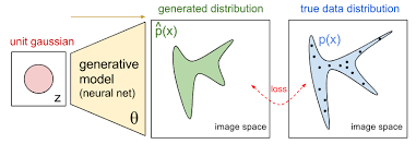
Bayesian Generative Modeling
- We want to model uncertainties in, say, images \(x\) (and maybe sample them), but these are very complicated objects
- We assume that each image \(x\) has some high-level features \(z\) that can help explain its uncertainty in a non-linear way \( p(x \mid f(z)) \ne p(x) \) where \(f\) is a neural network
- The features are believed to follow some simple distribution \(p(z)\)
- Having this model would allow us to
- Sample unseen images via \(z \sim p(z)\), \(x \sim p(x \mid z) \)
- Detect out-of-domain data using marginal density \(p(x)\)
INTRACTABLE
Bayesian Control Flow
- Suppose we have a residual neural network $$ H_l(x) = F_l(x) + x $$
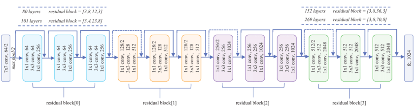
- Can we drop unnecessary computations for easy inputs?
- Lets equip the network with a mechanism to decide when to stop processing and prefer networks that stop early
Bayesian Control Flow
- Let \(z\) indicate the number of layers to use. Then $$H_l(x) = [z \le l] F_l(x) + x$$
- Thus we have $$p(y|x,z) = \text{Categorical}(y \mid \pi(x, z))$$ where \(\pi(x, z)\) is a residual network with \(z\) that controls when to stop processing the \(x\)
- We chose the prior on \(z\) s.t. lower values are more preferable
- How to decide upon number of layers at the test time?
- Obtain a sample from (or the mode statistic of) the true posterior $$ p(y, z \mid x) \propto p(y|x, z) p(z) $$
INTRACTABLE
Approximation Methods
Overcoming the intractability
Variational Inference
- We define some joint model \(p(y, \theta | x) = p(y | x, \theta) p(\theta) \)
- We obtain observations \( \mathcal{D} = \{ (x_1, y_1), ..., (x_N, y_N) \} \)
- We would like to infer possible values of \(\theta\) given observed data \(\mathcal{D}\) $$ p(\theta \mid \mathcal{D}) = \frac{p(\mathcal{D} | \theta) p(\theta)}{\int p(\mathcal{D}|\theta) p(\theta) d\theta} $$
- The denominator is generally intractable 😭
- We will be approximating true posterior distribution with an approximate one
- Need a distance between distributions to measure how good the approximation is $$ \text{KL}(q(x) || p(x)) = \mathbb{E}_{q(x)} \log \frac{q(x)}{p(x)} \quad\quad \textbf{Kullback-Leibler divergence}$$
- Not an actual distance, but \( \text{KL}(q(x) || p(x)) = 0 \) iff \(q(x) = p(x)\) for all \(x\) and is strictly positive otherwise
- Will be minimizing \( \text{KL}(q(\theta) || p(\theta | \mathcal{D})) \) over \(q\)
Variational Inference
- We'll take \(q(\theta)\) from some tractable parametric family, for example Gaussian $$ q(\theta | \Lambda) = \mathcal{N}(\theta \mid \mu(\Lambda), \Sigma(\Lambda)) $$
- Then we reformulate the objective s.t. we don't need the exact true posterior $$ \text{KL}(q(\theta | \Lambda) || p(\theta | \mathcal{D})) = \log p(\mathcal{D}) - \mathbb{E}_{q(\theta | \Lambda)} \log \frac{p(\mathcal{D}, \theta)}{q(\theta | \Lambda)} $$
- Hence we seek parameters \(\Lambda_*\) maximizing the following objective (the ELBO) $$ \Lambda_* = \text{argmax}_\Lambda \left[ \mathbb{E}_{q(\theta | \Lambda)} \log \frac{p(\mathcal{D}, \theta)}{q(\theta|\Lambda)} = \mathbb{E}_{q(\theta|\Lambda)} \log p(\mathcal{D}|\theta) - \text{KL}(q(\theta|\Lambda)||p(\theta)) \right]$$
- Once we find these, we get an approximate posterior predictive $$ q(y \mid x, \mathcal{D}) = \mathbb{E}_{q(\theta \mid \Lambda_*)} p(y \mid x, \theta) $$
- We can't compute this quantity analytically either, but can sample from \(q\) to get Monte Carlo estimates of the approximate posterior predictive distribution: $$ q(y \mid x, \mathcal{D}) \approx \hat{q}(y|x, \mathcal{D}) = \frac{1}{M} \sum_{m=1}^M p(y \mid x, \theta^m), \quad\quad \theta^m \sim q(\theta \mid \Lambda_*) $$
Gradient-Based Variational Inference
- Recall the objective for variational inference $$ \mathcal{L}(\Lambda_*) = \mathbb{E}_{q(\theta | \Lambda)} \log \frac{p(\mathcal{D}, \theta)}{q(\theta|\Lambda)} \to \max_{\Lambda} $$
- We'll be using well-known optimization method – Stochastic Gradient Descent
- We need (stochastic) gradient \(\hat{g}\) of \(\mathcal{L}(\Lambda)\) s.t. \(\mathbb{E} \hat{g} = \nabla_\Lambda \mathcal{L}(\Lambda) \)
- Problem: We can't just take \(\hat{g} = \nabla_\Lambda \log \frac{p(\mathcal{D}, \theta)}{q(\theta | \Lambda)} \) as the samples themselves depend on \(\Lambda\) through \(q(\theta|\Lambda)\)
- Remember the expectation is just an integral, and apply the log-derivative trick $$ \nabla_\Lambda q(\theta | \Lambda) = q(\theta | \Lambda) \nabla_\Lambda \log q(\theta|\Lambda) $$ $$ \nabla_\Lambda \mathcal{L}(\Lambda) = \int q(\theta|\Lambda) \log \frac{p(\mathcal{D}, \theta)}{q(\theta | \Lambda)} \nabla_\Lambda \log q(\theta | \Lambda) d\theta = \mathbb{E}_{q(\theta|\Lambda)} \log \frac{p(\mathcal{D}, \theta)}{q(\theta|\Lambda)} \nabla \log q(\theta | \Lambda) $$
- Though general, this gradient estimator has too much variance in practice
- Estimator is called REINFORCE, random search in disguise
Bayesian Neural Networks
Preferred Neural Networks
Bayesian Neural Networks
- We assume the data is generated using some (partially known) classifier \(\pi_{\theta}\): $$ p(y \mid x, \theta) = \text{Cat}(y | \pi_\theta(x)) \quad\quad \theta \sim p(\theta) $$
- True posterior is intractable $$ p(\theta \mid \mathcal{D}) \propto p(\theta) \prod_{n=1}^N p(y_n \mid x_n, \pi_\theta) $$
- Approximate it using \(q(\theta | \Lambda)\): $$ \Lambda_* = \text{argmax} \; \mathbb{E}_{q(\theta | \Lambda)} \left[\sum_{n=1}^N \log p(y_n | x_n, \theta) - \text{KL}(q(\theta | \Lambda) || p(\theta))\right] $$
- Essentially, instead of learning a single neural network that would solve the problem, we learn a distribution over networks that solve the problem – a (Bayesian) ensemble
- \(p(\theta)\) encodes our preferences on which networks we'd like to see
Dropout as a Bayesian Procedure
- Let \(q(\theta_i | \Lambda)\) be s.t. with some fixed probability \(p\) it's 0 and with probability \(1-p\) it's some learnable value \(\Lambda_i\)
- Then for some prior \(p(\theta)\) our optimization objective is $$ \mathbb{E}_{q(\theta|\Lambda)} \sum_{n=1}^N \log p(y_n | x_n, \theta) \to \max_{\Lambda} $$ where the KL term is missing due to the model choice
- No need to take special care about differentiating through samples
- We recover DropConnect
- The same can be done with dropout
- Turns out, these are bayesian approximate inference procedures
- What if we want to tune dropout rates \(p\)?
- Gradient-based optimization in discrete models is hard
- Invoke the Central Limit Theorem and turn the model into a continuous one
Sparse Bayesian Neural Networks
- Consider a model with continuous noise on weights $$ q(\theta_i | \Lambda) = \mathcal{N}(\theta_i | \mu_i(\Lambda), \alpha_i(\Lambda) \mu^2_i(\Lambda)) $$
- Neural Networks have lots of parameters, surely there's some redundancy in them
- Let's take a prior \(p(\theta)\) that would encourage large \(\alpha\)
- Large \(\alpha_i\) would imply that weight \(\theta_i\) is unbounded noise that corrupts predictions
- Such weights won't be doing anything useful, hence it should be zeroed out by putting \(\mu_i(\Lambda) = 0\)
- Thus the weight \(\theta_i\) would effectively turn into a deterministic 0
- Large \(\alpha\) encourage sparsification
- How do we backpropagate through samples \(\theta_i\)?
Reparametrization Trick
- We have a continuous density \(q(\theta_i | \mu_i(\Lambda), \sigma_i^2(\Lambda))\) and would like to compute the gradient of $$ \mathbb{E}_{q(\theta|\Lambda)} \log \frac{p(\mathcal{D}|\theta) p(\theta)}{q(\theta|\Lambda)} $$
- The gradient consists of two parts
- The inner part – expected gradients of \(\log \frac{p(\mathcal{D}|\theta) p(\theta)}{q(\theta|\Lambda)} \)
- This is easy
- Sampling part – gradients through samples \( \theta \sim q(\theta|\Lambda) \)
- The inner part – expected gradients of \(\log \frac{p(\mathcal{D}|\theta) p(\theta)}{q(\theta|\Lambda)} \)
- Reparametrization trick: replace a sample from \(q(\theta_i | \mu_i(\Lambda), \sigma_i^2(\Lambda))\) with a transformation of a sample from a parameter-less distribution: $$ \theta \sim \mathcal{N}(\mu, \sigma^2) \Leftrightarrow \theta = \mu + \sigma \varepsilon, \quad \varepsilon \sim \mathcal{N}(0, 1) $$
- The objective then becomes $$ \mathbb{E}_{\varepsilon \sim \mathcal{N}(0, 1)} \log \tfrac{p(\mathcal{D}, \mu + \varepsilon \sigma)}{q(\mu + \varepsilon \sigma | \Lambda)} $$
Sparsification in action
Variational Dropout Sparsifies Deep Neural Networks
D. Molchanov, A. Ashukha, D. Vetrov, ICML 2017
Bayesian Neural Networks: Conclusion
- The objective then becomes $$ \mathbb{E}_{\varepsilon \sim \mathcal{N}(0, 1)} \left[\sum_{n=1}^N \log p(y_n | \theta=\mu(\Lambda) + \varepsilon \sigma(\Lambda)) \right] - \text{KL}(q(\theta|\Lambda) || p(\theta)) $$
- Training a neural network with special kind of noise upon weights
- The magnitude of the noise is encouraged to increase
- Zeroes out unnecessary weights completely
- Essentially, training a whole ensemble of neural networks
- Actually using the ensemble is costly: \(k\) times slow for an ensemble of \(k\) models
- Single network (single-sample ensemble) also work
Bayesian Generative Models
Generating everything out of nothing
Bayesian Generative Models
- We assume the two-phase data-generating process:
- First, we decide upon high-level abstract features of the datum \(z \sim p(z)\)
- Then, we unpack these features using Neural Networks into an actual observable \(x\) using the (learnable) generator \(f_\theta\)
- This leads to the following model \(p(x, z) = p(x|z) p(z)\) where $$ p(x|z) = p(z) \prod_{d=1}^D p(x_d | f_\theta(z)) $$ $$ p(z) = \mathcal{N}(z | 0, I) $$ and \(f_\theta\) is some neural network
- We can sample new \(x\) by passing samples \(z\) through the generator once we learn it
- Would like to maximize log-marginal density of observed variables \(\log p(x)\)
- Intractable integral \( \log p(x) = \log \int p(x|z) p(z) dz \)
- Monte Carlo doesn't help much
Variational Inference to the rescue
- Introduce approximate posterior \(q(z|x)\): $$ q(z|x) = \mathcal{N}(z|\mu_\Lambda(x), \Sigma_\Lambda(x))$$
- Where \(\mu, \Sigma\) are generated using auxiliary inference network from the observation \(x\)
- Invoking the ELBO we obtain the following objective $$ \tfrac{1}{N} \sum_{n=1}^N \left[ \mathbb{E}_{q(z_n|x_n)} \log p(x_n | z_n) - \text{KL}(q(z_n|x_n)||p(z_n)) \right] \to \max_\Lambda $$
- Turns out, the ELBO is also a lower bound on marginal log-likelihood (hence the name), we can maximize it w.r.t. to parameters \(\theta\) of the generator also!
- Generator network and inference network essentially give us autoencoder
- Inference network encodes observations into latent code
- Generator network decodes latent code into observations
VAE
- Latent-variable Generative Model
- Generates observation from noise
- Can infer high-level abstract features of existing objects
- Useful for representation learning
- And semi-supervised learning
- Uses neural network to amortize inference
Auto-Encoding Variational Bayes
D. P Kingma, M. Welling, ICLR 2013
Conclusion
What this all was for
ConCLUSION
- Bayesian methods are useful when we have low data-to-parameters ratio
- The Deep Learning case!
- Bayesian methods can
- Impose useful priors on Neural Networks helping discover solutions of special form
- Provide better predictions
- Provide Neural Networks with uncertainty estimates (uncovered)
- Neural Networks help us make more efficient Bayesian inference
- Uses a lot of math
- Active area of research
Shameless Plug(s)
I sometimes blog about different cutting-edge-like topics: