presented by Artem Sobolev
Generative Modeling
- Given \(N\) samples from the true data-generating process \( p_\text{data}(x) \) and a model \( p_\theta(x) \)
- We'd like to find \( \hat\theta_N \) s.t. \( p_{\hat\theta_N}(x) \) is as close to \( p_\text{data}(x) \) as possible
- Typically we measure closeness by means of some divergence
- KL divergence
- MLE: VAEs, Flow-based models
- JS divergence, f-divergences, Wasserstein distance
- GANs
- KL divergence
Method of Moments
- Old and well-studied alternative to the Maximum Likelihood Estimation approach
- Moment function: \[ m(\theta) = \mathbb{E}_{p_\theta(x)} \Phi(x) \] where \( \Phi(x) \in \mathbb{R}^D \) -- some feature extractor
- Let \( \hat\theta_N \) be s.t. \[ m(\hat\theta_N) = \frac{1}{N} \sum_{n=1}^N \Phi(x_n) \]
- If \( p_\text{data}(x) = p_{\theta^\star}(x) \) for some \(\theta^\star\), then this estimator is consistent
Asymptotic Normality
- Theorem: if \( m(\theta) \) is a one-to-one mapping, and is continuously differentiable at \(\hat\theta_N\) with non-singular derivative \(\nabla_\theta \mathbb{E}_{p_\theta(x)} \Phi(x)\), assuming \(\mathbb{E}_{p_\theta(x)} \|\Phi(x)\|^2 < \infty\), \( \hat\theta_N \) exists with probability tending to 1, and satisfies \[ \sqrt{N}(\hat\theta_N - \theta^\star) \to \mathcal{N}\left(0, G^{-1} \Sigma G^{-T}\right), \quad\quad \Sigma = \text{Cov}_{p_\text{data}(x)} \; \Phi(x) \]
- Implications: some \( \Phi \) are better than others due to lower variance, and thus lower sample complexity
- Invertibility is too restrictive, can be relaxed to identifiability: \( m(\theta) = \mathbb{E}_{p_\text{data}(x)} \Phi(x)\) iff \(\theta = \theta^*\)
- Still hard to verify, instead assume \(G\) is full rank, and there are more moments than model parameters
Moment Networks
- It's hard to generate more moments than number of parameters in \(\theta\)
- Authors propose to use a moment network \(f_\phi(x)\) and let \[ \Phi(x) = [\nabla_\phi f_\phi(x), x, h_1(x), \dots, h_{L-1}(x)]^T \] where \(h_l(x)\) is activations of \(l\)-th layer
- Since moment function is not invertible anymore, the generator is trained by minimizing \[ \mathcal{L}^G(\theta) = \frac{1}{2} \left\| \frac{1}{N} \sum_{n=1}^N \Phi(x_n) - \mathbb{E}_{p(\varepsilon)} \Phi(g_\theta(\varepsilon)) \right\|_2^2 \]
Learning a Moment Network
- One could use a randomly initialized moment network \(f_\phi\)
- That would have large asymptotic variance of \(\hat\theta_N\)
- Ideally our \( \phi \) minimizes this asymptotic variance, which is approximately equivalent to maximizing \[ \| \mathbb{E}_{p(\varepsilon)} \Phi(g_\theta(\varepsilon)) - \mathbb{E}_{p_\text{data}(x)} \Phi(x) \|^2 \]
- However author claim that this maximization makes moments correlated, and breaks consistency of \(\hat\theta_N\)
- Authors follow prior work and introduce a binary classifier \[ \mathcal{L}^M(\phi) = \mathbb{E}_{p_\text{data}(x)} \log D_\phi(x) + \mathbb{E}_{p(\varepsilon)} \log (1-D_\phi(g_\theta(\varepsilon))) + \lambda R(x) \] where \( D_\phi(x) = \sigma(f_\phi(x)) \), and \(R\) regularizes \(\nabla_\phi f_\phi(x)\)
Nice Properties
- Asymptotic Normality assuming \(\mathcal{L}^G(\theta)\) is asymptotically quadratic \[ \sqrt{N} (\hat\theta_N - \theta^*) \to \mathcal{N}(0, V_{SE}) \]
- Even if we can't compute \( \mathbb{E}_{p(\varepsilon)} \Phi(g_\theta(\varepsilon)) \) analytically, and use Monte Carlo, this only increases asymptotic variance by a constant factor
- The method works for any \(\phi\), we only train it occasionally to increase sample efficiency
- Regularizes that controls asymptotic variance can be related to gradient penalty in WGANs
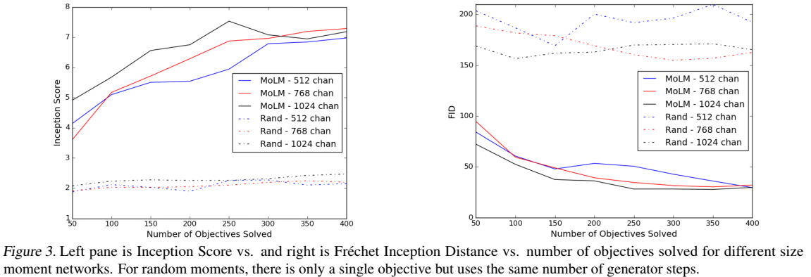
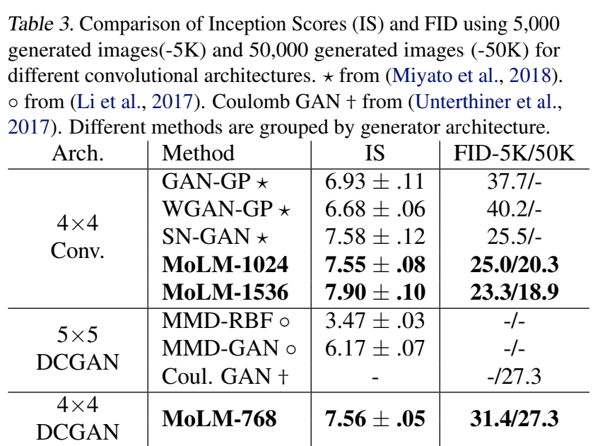
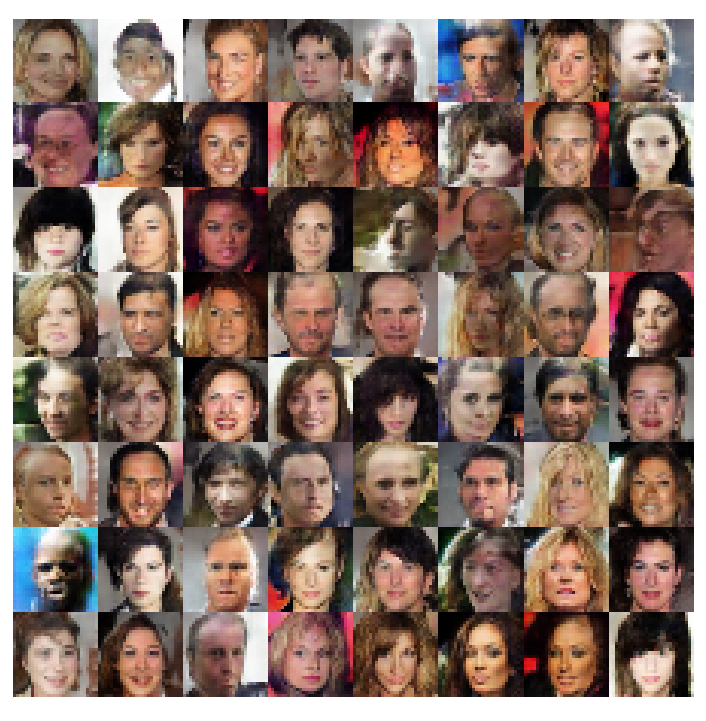
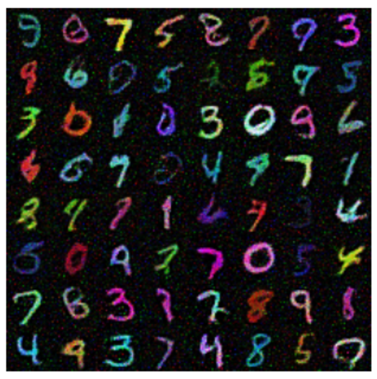
Experiments