Importance Weighted Hierarchical Variational Inference

Variational Inference

Suppose you're given a latent variable model, parametrized by $\theta$: $$ p_\theta(x) = \mathbb{E}_{p(z)} p_\theta(x|z) $$
Marginal log-likelihood is intractable, we thus resort to a lower bound: $$ \log p_\theta(x) \ge \mathbb{E}_{q_\phi(z|x)} \log \frac{p_\theta(x, z)}{q_\phi(z \mid x)} =: \text{ELBO} $$
Tightness of the bound is controlled by KL divergence between $q_\phi(z|x)$ and the true posterior $ p_\theta(z|x) $: $$ \log p_\theta(x) - \text{ELBO} = D_{KL}(q_\phi(z|x) \mid\mid p_\theta(z | x)) $$ $$ \text{ELBO} = \log p_\theta(x) - D_{KL}(q_\phi(z | x) \mid\mid p_\theta(z | x)) $$
Optimizing the ELBO w.r.t. $\phi$ leads to improving the proposal $q_\phi(z|x)$, hence the approximate posterior
Optimizing w.r.t. $\theta$ leads to a combination of increase in marginal log-likelihood and decrease in gap, making the true posterior and the model simpler

Variational Expressivity

Variational distributions $q_\phi(z|x)$ regularize the model, simple choices prevent the model $p_\theta(x, z)$ from having complicated dependence structure
Standard VAE[1] has a fully factorized Gaussian proposal
- Parameters are generated by an encoder aka an inference network
- Neural Networks amortize the inference, and do not increase expressiveness
- Gaussian proposal with full covariance matrix is still Gaussian
Can we leverage neural networks' universal approximation properties?

Neural Samplers as Proposals

Huston, we have a problem: we can sample such random variables, but can't evaluate output's density $$ \large \text{ELBO} := \mathbb{E}_{\color{green} q_\phi(z|x)} \log \frac{p_\theta(x,z)}{\color{red} q_\phi(z|x)} $$
There's been a huge amount of work on the topic

Invertible transformations with tractable Jacobians (Normalizing Flows)
- Theoretically appealing and shown to be very powerful
- Might require a lot of parameters, can't do abstraction
Methods that approximate the density ratio with a critic network
- Allow for fully implicit prior and proposal, handy in incremental learning
- Approximate nature breaks all bound guarantees
Give bounds on the intractable $ \log q_\phi(z|x) $
- Preserve the guarantees, but depend on bound's tightness

Hierarchical Proposals

From now on we will be considering Hierarchical Proposal of the form $$ q_\phi(z|x) = \int q_\phi(z | \psi, x) q_\phi(\psi | x) dz $$ Assume both distributions under the integral are easy to sample from and are reparametrizable
To keep the guarantees we need a lower bound on the ELBO: $$ \text{ELBO} = \mathbb{E}_{q_\phi(z|x)} \left[ \log p_\theta(x,z) - {\color{red} \log q_\phi(z|x)} \right] \; \ge \; ??? $$
Equivalently, we need an upper bound on the intractable term $\log q_\phi(z|x)$
- Standard variational bound would give a lower bound (leading to an upper bound on ELBO) 😞 $$ \log q_\phi(z|x) \ge \mathbb{E}_{\tau_\eta(\psi | x, z)} \log \frac{q(z, \psi | x)}{\tau_\eta(\psi|x,z)}, $$ $$\text{ELBO} \le \mathbb{E}_{q_\phi(z|x)} \mathbb{E}_{\tau_\eta(\psi|x,z)} \log \frac{p_\theta(x, z) \tau_\eta(\psi | x, z)}{q_\phi(z, \psi|x)} \stackrel{\not \ge}{\not \le} \log p_\theta(x) $$ where $\tau_\eta(\psi | x, z)$ is an auxiliary variational distribution with parameters $\eta$

Variational Upper Bound

Take a closer look at the obtained upper bound on ELBO, it's easy to make it a lower bound
Theorem: $$ \mathbb{E}_{q_\phi(z|x)} \mathbb{E}_{q_\phi(\psi|x,z)} \log \frac{p_\theta(x, z) \tau_\eta(\psi | x, z)}{q_\phi(z, \psi|x)} \le \text{ELBO} \le \log p_\theta(x) $$
Proof: Apply log and Jensen's inequality to this identity: $$ \mathbb{E}_{q_\phi(\psi | z, x)} \frac{\tau_\eta(\psi \mid x, z)}{q_\phi(z, \psi |x)} = \frac{1}{q_\phi(z|x)} \quad \Rightarrow \quad \mathbb{E}_{q_\phi(\psi | z, x)} \log \frac{\tau_\eta(\psi \mid x, z)}{q_\phi(z, \psi |x)} \le \log \frac{1}{q_\phi(z|x)}$$

That this gives a variational upper bound on marginal log-likelihood: $$ \log q_\phi(z|x) \le \mathbb{E}_{\color{blue} q_\phi(\psi|x, z)} \log \frac{q_\phi(z,\psi|x)}{\tau_\eta(\psi|x,z)} $$
- Notice the similarity with the standard variational lower bound $$ \log q_\phi(z|x) \ge \mathbb{E}_{\color{blue} \tau_\eta(\psi|x, z)} \log \frac{q_\phi(z,\psi|x)}{\tau_\eta(\psi|x,z)} $$
Merge $q_\phi(z) q_\phi(\psi|x,z)$ into $q_\phi(z, \psi|x)$, then factorize as $q_\phi(\psi|x) q_\phi(z|\psi, x)$

Q.E.D.

Hierarchical Variational Inference

So we just put VAE into the VAE $$ \mathbb{E}_{q_\phi(z, \psi|x)} \log \frac{p_\theta(x, z) \tau_\eta(\psi | x, z)}{q_\phi(z, \psi|x)} \le \log p_\theta(x) $$ Where the proposal $q_\phi(z|x)$ is a (conditional) latent variable model itself!
Another way to look at this bound is as if we augmented the generative model $p_\theta(x, z)$ with an auxiliary distribution $\tau_\eta(\psi|x,z)$ and then performed joint variational inference for $z, \psi$
Thus the name auxiliary variables[2] aka hierarchical variational model[3]
However, now we have a similar problem, the gap with the ELBO is $$ \text{ELBO} - \mathbb{E}_{q_\phi(z, \psi|x)} \log \frac{p_\theta(x, z) \tau_\eta(\psi | x, z)}{q_\phi(z, \psi|x)} = D_{KL}(q_\phi(\psi|x,z) \mid\mid \tau_\eta(\psi|x,z)) $$
So even though $q_\phi(z|x)$ is allowed to be a complicated hierarchical model, this bound favors simple models with $q_\phi(\psi|z,x)$ being close to $\tau_\eta(\psi|x,z)$
Besides, $q_\phi(z, \psi|x)$ might disregard the auxiliary r.v. $\psi$ and degenerate to a simple parametric model, indicated by $q_\phi(\psi|x, z) = q_\phi(\psi|x)$

Multisample Lower Bounds Recap

The standard ELBO admits tightening through usage of multiple samples: $$ \text{ELBO} \le \text{IW-ELBO}_M := \mathbb{E}_{q_\phi(z_{1:M}|x)} \log \frac{1}{M} \sum_{m=1}^M \frac{p_\theta(x, z_m)}{q_\phi(z_m|x)} \le \log p_\theta(x) $$
Known as Importance Weighted Variational Inference[4,5]
Can be interpreted[5] as a refining procedure that improves the standard proposal $q_\phi(z|x)$, turning it into $\hat{q}_\phi^M$:
1. Sample M i.i.d. $z$ from the $q_\phi(z|x)$
2. For each one compute its ELBO $w_k = \log p(x, z_m) - \log q_\phi(z_m)$
3. Sample $h \sim \text{Categorical}(\text{softmax}(w)) $
4. Return $z_h$
Except... the ELBO with such proposal would be hard to compute and optimize over, so the IWAE objective turns out to be a lower bound on that: $$ \text{ELBO}[q_\phi] \le \text{IW-ELBO}_M[q_\phi] \le \text{ELBO}[\hat{q}_\phi^M] $$
Requires $M$ high-dimensional decoder $p_\theta(x, z_m)$ evaluations

Multisample Upper Bounds?

Can we tighten the variational upper bound using multiple samples?
Sure! $$ \mathbb{E}_{q_\phi(\psi_{1:M} | z, x)} \frac{1}{M} \sum_{m=1}^M \frac{\tau_\eta(\psi \mid x, z)}{q_\phi(z, \psi |x)} = \frac{1}{q_\phi(z|x)} \quad $$ Thus $$ \mathbb{E}_{q_\phi(\psi_{1:M} | z, x)} \log \frac{1}{M} \sum_{m=1}^M \frac{\tau_\eta(\psi \mid x, z)}{q_\phi(z, \psi |x)} \le \log \frac{1}{q_\phi(z|x)}$$ And $$ \log q_\phi(z|x) \le \mathbb{E}_{q_\phi(\psi_{1:M} | z, x)} \log \frac{1}{\frac{1}{M} \sum_{m=1}^M \frac{\tau_\eta(\psi \mid x, z)}{q_\phi(z, \psi |x)}} $$
But is this bound practical? Hell, no.
- It requires sampling from the true posterior not once, but $M$ times!
- A variational Harmonic estimator, which is known[6] to behave very poorly

A case of Semi-Implicit VI

Curiously, Semi-Implicit Variational Inference[7] proposed the following lower bound on the ELBO: $$ \mathbb{E}_{q_\phi(z, \psi_0|x)} \mathbb{E}_{\color{blue} q_\phi(\psi_{1:K}|x)} \log \frac{p_\theta(x, z)}{\color{blue} \frac{1}{K+1} \sum_{k=0}^K q_\phi(z|x, \psi_k)} \le \text{ELBO}[q_\phi] \le \log p_\theta(x) $$
Equivalently, $$ \log q_\phi(z|x) \le \mathbb{E}_{q_\phi(\psi_0|x, z)} \mathbb{E}_{\color{blue} q_\phi(\psi_{1:K}|x)} \log \frac{1}{K+1} \sum_{k=0}^K q_\phi(z|\psi_k, x) $$
Recall the lower variational multisample bound: $$ \log q_\phi(z|x) \ge \mathbb{E}_{\color{blue} \tau_\eta(\psi_{1:K}|z,x)} \log \frac{1}{K} \sum_{k=1}^K \frac{q_\phi(z,\psi_k|x)}{\tau_\eta(\psi_k|x,z)} $$or, for $\tau_\eta(\psi|x,z) = q_\phi(\psi|x)$: $$ \log q_\phi(z|x) \ge \mathbb{E}_{\color{blue} q_\phi(\psi_{1:K}|x)} \log \frac{1}{K} \sum_{k=1}^K q_\phi(z|\psi_k, x) $$

These two look suspiciously similar!

Are we onto something?

So, we know that the following is an upper bound for at least one particular choice of $\tau_\eta(\psi|x,z)$ $$ \mathbb{E}_{q_\phi(\psi_0|x, z)} \mathbb{E}_{\color{red} \tau_\eta(\psi_{1:K}|z,x)} \log \frac{1}{K+1} \sum_{k=0}^K \frac{q_\phi(z,{\color{red}\psi_k}| x)}{\color{red} \tau_\eta(\psi_k \mid x, z)} \quad\quad (1) $$
Moreover, for $K=0$ it reduces to the already discussed HVM bound, also an upper bound: $$ \log q_\phi(z | x) \le \mathbb{E}_{q_\phi(\psi_0|x, z)} \log \frac{q_\phi(z,\psi_0| x)}{\tau_\eta(\psi_0 \mid x, z)} $$
Finally, for $\tau_\eta(\psi|x,z) = q_\phi(\psi|x,z)$ we exactly recover $\log q_\phi(\psi|x,z)$

Given all this evidence, it's time to question ourselves: Is this all just a coincidence? Or, is the (1) indeed a multisample $\tau$-variational upper bound on the marginal log-density $\log q_\phi(z|x)$?

Multisample Variational Upper Bound Theorem

Theorem: for $K \in \mathbb{N}_0 $, any* $q_\phi(z, \psi|x)$ and $\tau_\eta(\psi|x,z)$ denote $$ \mathcal{U}_K := \mathbb{E}_{q_\phi(\psi_0|x, z)} \mathbb{E}_{\tau_\eta(\psi_{1:K}|z,x)} \log \frac{1}{K+1} \sum_{k=0}^K \frac{q_\phi(z,\psi_k| x)}{\tau_\eta(\psi_k \mid x, z)}$$Then the following holds

$\mathcal{U}_K \ge \log q_\phi(z|x)$
$\mathcal{U}_K \ge \mathcal{U}_{K+1} $
$\lim_{K \to \infty} \mathcal{U}_K = \log q_\phi(z|x) $

Proof: we will only prove the first statement by showing that the gap between the bound and the marginal log-density is equal to some KL divergence

Proof of Multisample Variational Upper Bound Theorem

Proof: consider the gap $$ \mathbb{E}_{q_\phi(\psi_0|x, z)} \mathbb{E}_{\tau_\eta(\psi_{1:K}|z,x)} \log \tfrac{1}{K+1} \sum_{k=0}^K \frac{q_\phi(z,\psi_k| x)}{\tau_\eta(\psi_k \mid x, z)} - \log q_\phi(z|x)$$

Multiply and divide by $q_\phi(\psi_0|x,z) \tau_\eta(\psi_{1:K}|x,z)$ to get $$ \mathbb{E}_{q_\phi(\psi_0|x, z)} \mathbb{E}_{\tau_\eta(\psi_{1:K}|z,x)} \log \frac{q_\phi(\psi_0|x, z) \tau_\eta(\psi_{1:K}|z,x)}{\frac{q_\phi(\psi_0|x, z) \tau_\eta(\psi_{1:K}|z,x)}{\tfrac{1}{K+1} \sum_{k=0}^K \frac{q_\phi(\psi_k| z,x)}{\tau_\eta(\psi_k \mid x, z)}}} $$

Subtract the log $$ \mathbb{E}_{q_\phi(\psi_0|x, z)} \mathbb{E}_{\tau_\eta(\psi_{1:K}|z,x)} \log \tfrac{1}{K+1} \sum_{k=0}^K \frac{q_\phi(\psi_k| z,x)}{\tau_\eta(\psi_k \mid x, z)} $$

Which is exactly the KL divergence $$ D_{KL}\left(q_\phi(\psi_0|x, z) \tau_\eta(\psi_{1:K}|z,x) \mid\mid \frac{q_\phi(\psi_0|x, z) \tau_\eta(\psi_{1:K}|z,x)}{\tfrac{1}{K+1} \sum_{k=0}^K \frac{q_\phi(\psi_k| z,x)}{\tau_\eta(\psi_k \mid x, z)} }\right)$$

Is the second argument even a distribution?

For the KL to enjoy non-negativity and be 0 when distributions match, we need the second argument to be a valid probability density. Is it? $$ \omega_{q,\tau}(\psi_{0:K}|x,z) := \frac{q_\phi(\psi_0|x, z) \tau_\eta(\psi_{1:K}|z,x)}{\tfrac{1}{K+1} \sum_{k=0}^K \frac{q_\phi(\psi_k| z,x)}{\tau_\eta(\psi_k \mid x, z)} }$$

We'll show it by means of symmetry:

$$ \int \frac{q_\phi(\psi_0|x, z) \tau_\eta(\psi_{1:K}|z,x)}{\tfrac{1}{K+1} \sum_{k=0}^K \frac{q_\phi(\psi_k| z,x)}{\tau_\eta(\psi_k \mid x, z)} } d\psi_{0:K} = \int \frac{\frac{q_\phi(\psi_0|x, z)}{\tau_\eta(\psi_0|x, z)} \tau_\eta(\psi_{0:K}|z,x)}{\tfrac{1}{K+1} \sum_{k=0}^K \frac{q_\phi(\psi_k| z,x)}{\tau_\eta(\psi_k \mid x, z)} } d\psi_{0:K} =$$

However, there's nothing special in the choice of the 0-th index, we could take any $j$ and the expectation wouldn't change. Let's average all of them: $$= \int \frac{\frac{q_\phi(\psi_j|x, z)}{\tau_\eta(\psi_j|x, z)} \tau_\eta(\psi_{0:K}|z,x)}{\tfrac{1}{K+1} \sum_{k=0}^K \frac{q_\phi(\psi_k| z,x)}{\tau_\eta(\psi_k \mid x, z)} } d\psi_{0:K} = \frac{1}{K+1} \sum_{j=0}^K \int \frac{\frac{q_\phi(\psi_j|x, z)}{\tau_\eta(\psi_j|x, z)} \tau_\eta(\psi_{0:K}|z,x)}{\tfrac{1}{K+1} \sum_{k=0}^K \frac{q_\phi(\psi_k| z,x)}{\tau_\eta(\psi_k \mid x, z)} } d\psi_{0:K}$$

Q.E.D.

$$ = \int \frac{\frac{1}{K+1} \sum_{j=0}^K \frac{q_\phi(\psi_j|x, z)}{\tau_\eta(\psi_j|x, z)} \tau_\eta(\psi_{0:K}|z,x)}{\tfrac{1}{K+1} \sum_{k=0}^K \frac{q_\phi(\psi_k| z,x)}{\tau_\eta(\psi_k \mid x, z)} } d\psi_{0:K} = \int \tau_\eta(\psi_{0:K}|z,x) d\psi_{0:K} = 1$$

Toy Example

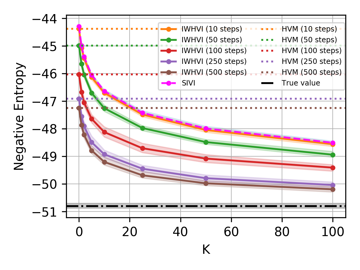
Lets see how our variational upper bound compares with prior work.

Consider standard D-dim. Laplace distribution as a scale-mixture of Normals: $$ q(z) = \int \prod_{d=1}^D \mathcal{N}(z^{(d)}|0, \psi^{(d)}) \text{Exp}(\psi^{(d)} \mid \tfrac{1}{2}) d\psi^{(1:D)} $$
To test bound's behavior in high dimensions we won't be using the factorization property.
As a proposal $\tau(\psi \mid z)$ we will use a Gamma distribution whose parameters are generated by a neural network with three hidden layers of size $10 D$
We give an upper bound on negative differential entropy: $$ \mathbb{E}_{q(z)} \log q(z) \le \mathbb{E}_{q(z, \psi_0)} \mathbb{E}_{\text{Gamma}(\psi_{1:K}|\alpha(z), \beta(z))} \log \tfrac{1}{K+1} \sum_{k=0}^K \tfrac{\prod_{d=1}^D \mathcal{N}(z^{(d)}|0, \psi_k^{(d)})\text{Exp}(\psi_k^{(d)}|\tfrac{1}{2})}{\prod_{d=1}^D \text{Gamma}(\psi_k^{(d)} |\alpha(z)_d, \beta(z)_d)} $$
We initialize auxiliary inference network s.t. untrained network produces $\alpha(z) \approx 1$ and $\beta(z) \approx \tfrac{1}{2}$, collapsing into the $\text{Exp}(\tfrac{1}{2})$ prior, and giving us the SIVI bound

Toy Example

Multisample Variational Sandwich Bounds on KL

Corollary: for the case of two hierarchical distributions $q(z) = \int q(z, \psi) d\psi $ and $p(z) = \int p(z, \zeta) d\zeta $, we can give the following multisample variational bounds on KL divergence:

$$ \large D_{KL}(q(z) \mid\mid p(z)) \le \mathbb{E}_{q(z, \psi_0)} \mathbb{E}_{\tau(\psi_{1:K}|z)} \mathbb{E}_{\nu(\zeta_{1:L}|z)} \log \frac{\tfrac{1}{K+1} \sum_{k=0}^K \frac{q(z, \psi_k)}{\tau(\psi_k|z)}}{\frac{1}{L} \sum_{l=1}^L \frac{p(z, \zeta_l)}{\nu(\zeta_l|z)} } $$

$$ \large D_{KL}(q(z) \mid\mid p(z)) \ge \mathbb{E}_{q(z)} \mathbb{E}_{\tau(\psi_{1:K}|z)} \mathbb{E}_{p(\zeta_0|z)} \mathbb{E}_{\nu(\zeta_{1:L}|z)} \log \frac{\tfrac{1}{K} \sum_{k=1}^K \frac{q(z, \psi_k)}{\tau(\psi_k|z)}}{\frac{1}{L+1} \sum_{l=0}^L \frac{p(z, \zeta_l)}{\nu(\zeta_l|z)} } $$

Where $\tau(\psi|z)$ and $\nu(\zeta|z)$ are variational approximations to $q(\psi|z)$ and $p(\zeta|z)$, correspondingly

Note: actually, variational distributions in the lower and upper bounds optimize different divergences, thus technically they should be different

ELBO with Hierarchical Proposal

We can now combine KL's upper bound with ELBO to obtain a lower bound: $$ \mathbb{E}_{q(z, \psi_{0}|x)} \mathbb{E}_{\tau_\eta(\psi_{1:K}|x,z)} \log \frac{p_\theta(x, z)}{\frac{1}{K+1} \sum_{k=0}^K \frac{q_\phi(z, \psi_{k}|x)}{\tau_\eta(\psi_{k}|z, x)} } \le \log p_\theta(x) $$ Called Importance Weighted Hierarchical Variational Inference bound
Semi-Implicit Variational Inference bound obtained for $\tau(\psi|x,z) = q_\phi(\psi|x) $: $$ \mathbb{E}_{q(z, \psi_{0}|x)} \mathbb{E}_{q_\phi(\psi_{1:K}|x)} \log \frac{p_\theta(x, z)}{\frac{1}{K+1} \sum_{k=0}^K q_\phi(z | \psi_{k}, x) } \le \log p_\theta(x) $$
Hierarchical Variational Models bound obtained by setting $K = 0$: $$ \mathbb{E}_{q(z, \psi|x)} \log \frac{p_\theta(x, z)}{ \frac{q_\phi(z, \psi|x)}{\tau_\eta(\psi|z, x)} } = \mathbb{E}_{q(z, \psi|x)} \log \frac{p_\theta(x, z) \tau_\eta(\psi|z, x)}{ q_\phi(z, \psi|x) } \le \log p_\theta(x) $$
- The Joint bound obtained by implicitly setting $\tau_\eta(\psi|x,z) = p_\theta(\psi|x,z)$: $$ \mathbb{E}_{q(z, \psi|x)} \log \frac{p_\theta(x, z)}{ \frac{q_\phi(z, \psi|x)}{p_\theta(\psi|z, x)} } = \mathbb{E}_{q(z, \psi|x)} \log \frac{p_\theta(x, z, \psi)}{ q_\phi(z, \psi|x) } \le \log p_\theta(x) $$

Comparison to Prior Bounds

SIVI allows for unknown mixing density $q_\phi(\psi|x)$ as long as we can sample
- $q_\phi(\psi|x)$ is assumed to be implicit and reprametrizable, therefore we can reformulate the model to have an explicit "prior": $$ q_\phi(z|x) = \int q_\phi(z|\psi, x) q_\phi(\psi|x) d\psi \quad\Rightarrow\quad q_\phi(z|x) = \int q_\phi(z|\psi(\varepsilon; \phi), x) q(\varepsilon) d\varepsilon $$
- We thus can assume we know $\psi$'s density in most cases
IWHVI needs to make an extra pass of $z$ through $\tau$'s network to generate the $\tau$ distribution, however it's dominated by multiple $q_\phi(z, \psi_k|x)$ evaluations, needed for both SIVI and IWHVI
SIVI's poor choice of $q_\phi(\psi|x)$ as an auxiliary variational approximation of $q_\phi(\psi|x,z)$ leads to samples $\psi$ that are uninformed about the current $z$ and miss the high probability area of $\psi|z$, essentially leading to random guesses
HVM also uses the targeted auxiliary variational approximation, but lacks multisample tightening, leading to heavier penalization for complex $q_\phi(\psi|x,z)$

Multisample ELBO with Hierarchical Proposal

So far we used multiple samples of $\psi$ to tighten the $\log q_\phi(z|x)$ bound
But we can also use multiple samples of $z$ to tighten the $\log p_\theta(x)$ bound $$ \mathbb{E}_{q(z_{1:M}, \psi_{1:M,0}|x)} \mathbb{E}_{\tau_\eta(\psi_{1:M,1:K}|x,z_{1:M})} \log \frac{1}{M} \sum_{m=1}^M \frac{p_\theta(x, z_m)}{\frac{1}{K+1} \sum_{k=0}^K \frac{q_\phi(z_m, \psi_{mk}|x)}{\tau_\eta(\psi_{mk}|z_m, x)} } \le \log p_\theta(x) $$ Called Doubly Importance Weighted Hierarchical Variational Inference bound
This bound requires $O(M + M K)$ samples of $\psi$
Interestingly, SIVI allows for sample reuse, needing only $O(M+K)$ samples: $$ \mathbb{E}_{q(z_{1:M}, \psi_{1:M}|x)} \mathbb{E}_{q_\phi(\psi_{M+1:M+K}|x)} \log \frac{1}{M} \sum_{m=1}^M \frac{p_\theta(x, z_m)}{\frac{1}{M+K} \sum_{k=1}^{M+K} q_\phi(z_m| \psi_{k},x) } \le \log p_\theta(x) $$
- Same trick cannot be applied to the DIWHVI
- One possible solution is to consider a multisample-conditioned proposal $\tau_\eta(\psi|z_{1:M})$ that is invariant to any permutation of $z_{1:M}$

VAE Experiment

We used the DIWHVI bound: $$ \mathbb{E}_{q(z_{1:M}, \psi_{1:M,0}|x)} \mathbb{E}_{\tau_\eta(\psi_{1:M,1:K}|x,z_{1:M})} \log \frac{1}{M} \sum_{m=1}^M \frac{p_\theta(x, z_m)}{\frac{1}{K+1} \sum_{k=0}^K \frac{q_\phi(z_m, \psi_{mk}|x)}{\tau_\eta(\psi_{mk}|z_m, x)} } \le \log p_\theta(x) $$
For training we used $M=1$ and gradually increased $K$ from 1 to 50
For evaluation we used $M=5000$ and $K=100$
- For SIVI we trained $\tau_\eta(\psi|x,z)$ separately after the model was trained
$p_\theta(x|z)$ was generated by a neural network with two hidden layers of size $H$
$q_\phi(z|x, \psi)$ was generated by a neural network with two hidden layers of size $H$, but in addition $\psi$ was concatenated with all intermediate representations
$q(\psi|x)$ was standard Normal distribution, independent of $x$
$\tau_\eta(\psi|x,z)$ was generated by a neural network with two hidden layers of size $H$ and took concatenated $(x, z)$ vector as input

VAE Experiment

Method	MNIST	OMNIGLOT
AVB+AC	−83.7 ± 0.3	—
IWHVI	−83.9 ± 0.1	−104.8 ± 0.1
SIVI	−84.4 ± 0.1	−105.7 ± 0.1
HVM	−84.9 ± 0.1	−105.8 ± 0.1
VAE+RealNVP	−84.8 ± 0.1	−106.0 ± 0.1
VAE+IAF	−84.9 ± 0.1	−107.0 ± 0.1
VAE	−85.0 ± 0.1	−106.6 ± 0.1

Test log-likelihood on dynamically binarized MNIST and OMNIGLOT with 2 std. interval

The Signal-to-Noise Ratio Problem of Tighter Bounds

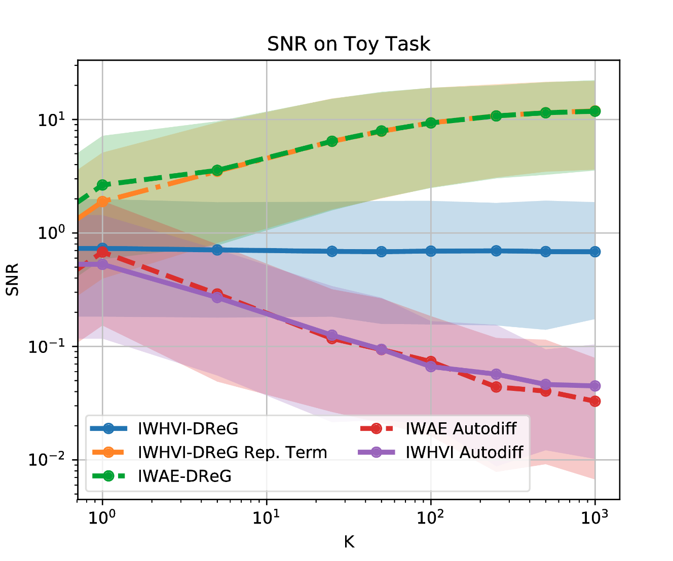
For IWAE it was shown[8] that the quality (as measured by the signal-to-noise ratio) of the gradients w.r.t. $\theta$ increases with $M$, but SNR of the gradients w.r.t. $\phi$ decreases.
- Increasing $M$ increases noise in $\nabla_\phi$, undermining the inference network
- The same problem, if exists in our case, might prevent us from learning good $\tau$, diminishing our advantage over SIVI
Luckily, it was recently shown[9] that the source of this high variance is a hidden REINFORCE-like term in the (reparametrized!) gradient estimator, and it can be removed by a second application of the reparametrization trick.

The same reasoning can be applied to our bound. It does, indeed, contain a REINFORCE-like term in the reparametrized gradient estimator, which hurts the SNR, but can be similarly removed by the 2nd reparametrization

The Signal-to-Noise Ratio Problem of Tighter Bounds

Debiasing

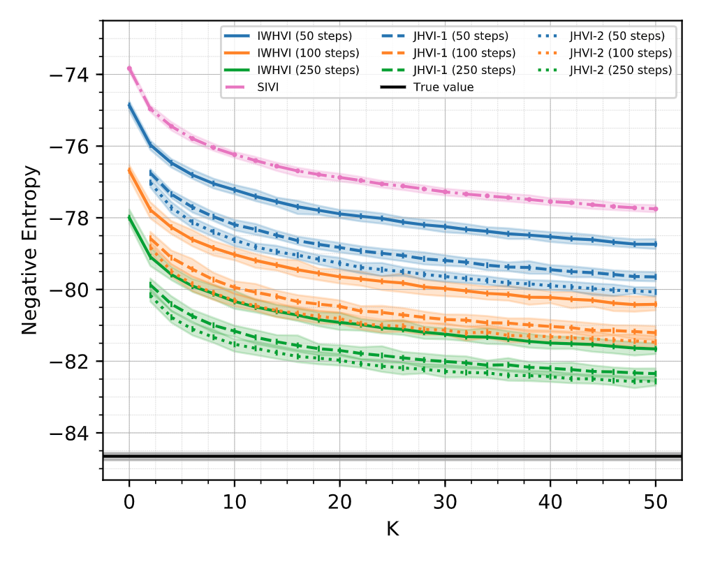
IWAE bound can be seen as a biased evidence $\log p_\theta(x)$ approximator. The bias can can be shown to be of order $O(1/M)$: $$ \log p_\theta(x) - \mathbb{E}_{q_\phi(z_{1:M}|x)} \log \frac{1}{M} \sum_{m=1}^M \frac{p_\theta(x, z_m)}{q_\phi(z_m)} = \frac{\alpha_1}{M} + O\left(\tfrac{1}{M^2}\right) $$
One can apply Jackknife to reduce the bias to $O(1/M^2)$
By applying Jackknife D times one gets[10] bias of order $O(1/M^{D+1})$
However, such "debiased" estimator is not guaranteed to be a lower bound

Same trick is possible for the IWHVI to get tighter estimates of the marginal log-likelihood that tend to overestimate $\log p_\theta(x)$

Debiasing Experiment

Conclusion

We presented a variational multisample lower bound on the intractable ELBO for the case of a hierarchical proposal $q_\phi(z|x)$
The bound turned out to generalize many previous methods
- Most importantly, it bridges HVM and SIVI
We showed that the proposed bound improves upon its special cases
- It is a tighter upper bound on the marginal log-density $\log q_\phi(z|x)$
- It reduces regularizational effect of the auxiliary variational distributions of both SIVI and HVM, allowing for more expressive marginal $q_\phi(z|x)$
It is closely related to IWAE, and many results apply to the IWHVI as well
- It benefits from double reparametrization to improve gradients
- The gap can be reduced by means of the Jackknife
- IWHVI can be combined with IWAE to obtain an even tighter lower bound on the marginal log-likelihood $\log p_\theta(x)$
... it is not yet fully understood

References

Auto-Encoding Variational Bayes by Diederik P Kingma and Max Welling
Auxiliary Deep Generative Models by Lars Maaløe, Casper Kaae Sønderby, Søren Kaae Sønderby, Ole Winther
Hierarchical Variational Models by Rajesh Ranganath, Dustin Tran, David M. Blei
Importance Weighted Autoencoders by Yuri Burda, Roger Grosse, Ruslan Salakhutdinov
Importance Weighting and Variational Inference by Justin Domke and Daniel Sheldon
The Harmonic Mean of the Likelihood: Worst Monte Carlo Method Ever by Radford Neal
Semi-Implicit Variational Inference by Mingzhang Yin and Mingyuan Zhou
Tighter Variational Bounds are Not Necessarily Better by Tom Rainforth, Adam R. Kosiorek, Tuan Anh Le, Chris J. Maddison, Maximilian Igl, Frank Wood, Yee Whye Teh
Doubly Reparameterized Gradient Estimators for Monte Carlo Objectives by George Tucker, Dieterich Lawson, Shixiang Gu, Chris J. Maddison
Debiasing Evidence Approximations: On Importance-weighted Autoencoders and Jackknife Variational Inference by Sebastian Nowozin