
Causal Inference
Hui Hu Ph.D.
Department of Epidemiology
College of Public Health and Health Professions & College of Medicine
November 8, 2018
PHC6016 Social Epidemiology
Theory
IP Weighting and Marginal Structural Models
Standardization and Parametric G-Formula
Theory
Individual Causal Effects
- Zeus is a patient waiting for a heart transplant
- on Jan 1, he receives a new heart
- five days later, he dies - Another patient, Hera
- she also received a heart transplant on Jan 1
- five days later she was alive
Treatment: A (1: treated, 0: untreated)
Outcome: Y (1: death, 0: survival)
Potential outcomes or counterfactual outcomes:
Y a=0 : the outcome variable that would have been observed under the treatment value a=0.
Y a=1 : the outcome variable that would have been observed under the treatment value a=1.
Definition of individual causal effects: the treatment A has a causal effect on an individual's outcome Y if Y a=1 ≠ Y a=0 for the individual.
Y a=1 =1
Ya=1=0
In general, individual causal effects cannot be identified since only one of potential outcomes is observed for each individual.
Average Causal Effects
Definition of average causal effects: an average causal effect of treatment A on outcome Y is present if E[ Y a=1 ] ≠ E[ Y a=0 ]
Pr[ Y a=1 =1]=10/20=0.5
Absence of an average causal effect does not imply absence of individual effects.

Pr[ Y a=0 =1]=10/20=0.5
Average causal effects can sometimes be identified from data even if individual causal effects cannot.
Causation vs. Association
Pr[ Y a =1]

Pr[ Y=1|A=a]
Marginal probability
Conditional probability
Causation vs. Association

- Causal inference requires data like the hypothetical first table, but all we can ever expect to have is real world data like those in the second table.
- Under which conditions real world data can be used for causal inference?
Randomization

- Randomization ensures that those missing values occurred by chance
- Ideal randomized experiment
- no loss to follow-up
- full adherence to treatment
- a single version of treatment
- double blind assignment - Exchangeability:
- which particular group received the treatment is irrelevant for the value of Pr[ Ya=1|A=1] and Pr[ Ya=1|A=0]


Randomization is so highly valued because it is expected to produce exchangeability.
Randomization
- Does exchangeability hold in our heart transplant study?
-
- Since the counterfactual data are not available in the real world, we are generally unable to determine whether exchangeability holds


1
0
0
0
1
0
1
0
1
0
0
1
1
0
0
0
1
1
1
1
Can we conclude that our study is not a randomized experiment?
- random variability
- conditional randomization
Conditional Randomization

- Prognosis factor L (1: critical condition, 0 otherwise)
- Design 1
- randomly assign treatments to 65% of the individuals
- Design 2
- randomly assign treatments to 75% of the individuals with critical condition
- randomly assign treatments to 50% of those in noncritical condition
Marginal randomization
Conditional randomization
Exchangeability holds
Exchangeability does not hold, but conditional exchangeability holds


How to compute the causal effect?
- Stratum-specific causal effects
- Average causal effects
Standardization
Inverse Probability Weighting


Since
Similarly,


Causal Inference for Observational Study
What randomized experiment are we trying to emulate?
Observational Study
- An observational study can be conceptualized as a conditionally randomized experiment under the following 3 conditions (also called identifiability conditions):
- exchangeability: the conditional probability of receiving every value of treatment, though not decided by the investigators, depends only on the measured covariates
- positivity: the conditional probability of receiving every value of treatment is greater than zero
- consistency: the values of treatment under comparison correspond to well-defined interventions that, in turn, correspond to the versions of treatment in the data
- When any of these conditions does not hold, another possible approach can be used:
- instrumental variable: a predictor of treatment, which was hoped to be randomly assigned conditional on the measured covariates
Exchangeability
- The crucial question for the observational study is whether L is the only outcome predictor that is unequally distributed between the treated and the untreated
- In the absence of randomization, there is no guarantee that conditional exchangeability holds
- When we analyze an observational study under the assumption of conditional exchangeability, we must hope that the assumption is at least approximately true

Positivity
- With all the subjects receiving the same treatment level, computing the average causal effect would be impossible
- In observational studies, positivity is not guaranteed, but it can sometimes be empirically verified


Consistency
- For observational studies, we assume that the treatment of interest either does not have multiple versions, or has multiple versions with identical effects
- An example:
- an obese individual (R=1) who died (Y=1)
- multiple versions A(r=0) of the treatment R=0 (e.g. more exercise, less food intake, more cigarette smoking, genetic modification, bariatric surgery, etc.)
- the counterfactual outcome Y is not well defined
- a nonobese individual might have died if he had been nonobese through cigarette smoking (lung cancer), and might have survived if through a better diet - In settings with ill-defined interventions, the consistency condition does not hold because the counterfactual outcome Y may not equal the observed outcome Y in some people with R=r
r=0
r
IP Weighting and Marginal Structural Models
-
National Health and Nutrition Examination Survey Data I Epidemiologic Follow-up Study
- To estimate the average causal effect of smoking cessation A on weight gain Y
- 1,566 cigarette smokers aged 25-74 years
- with a baseline visit and a follow-up visit 10 years later
- A=1 if reported having quit smoking before the follow-up visit, and A=0 otherwise
- weight gain Y was measured as the body weight at the follow-up visit minus the body weight at the baseline visit


Data


Assume these 9 baseline variables are sufficient to adjust for confounding

Estimating IP weights via modeling
- IP weighting creates a pseudo-population in which the arrow from the confounders L to the treatment A is removed
- The pseudo-population is created by weighting each individual by the inverse of the conditional probability of receiving the treatment level that one indeed received
-
- Fit a logistic regression model for the probability of quitting smoking with all 9 confounders included as covariates
- Compute the difference in the pseudo-population created by the estimated IP weights


= {


quitters
non-quitters


Estimating IP weights via modeling

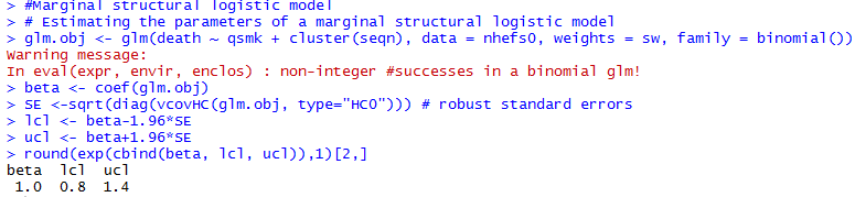
Fit the linear model by weighted least squares, with individuals weighted by their estimated IP weights
To obtain a 95% confidence interval:
- to use statistical theory to derive the corresponding variance estimator (not available in most software)
- approximate the variance by bootstrapping (time-consuming)
- use the robust variance estimator (widely available, quick, but generate conservative CI)


Stabilized IP Weights
- The goal of IP weighting is to create a pseudo-population in which there is no association between the covariates L and treatment A
- all individuals have the same probability of receiving A=1 and the same probability of receiving A=0 - The pseudo-population was twice as large as the study population because all individuals were included both under treatment and under no treatment
- Equivalently, the expected mean of the weights was 2
- There are other ways to create a pseudo-population:

f(A) equals to Pr[A=1] for treated, and Pr[A=0] for untreated

Marginal Structural Models
- The outcome variable of this model is counterfactual
- Models for mean counterfactual outcomes are referred to as structural mean models
- when it does not include any covariates, we refer to it as an unconditional or marginal structural mean model - The parameters for treatment in structural models correspond to average causal effects
- The above model is saturated because smoking cessation A is a dichotomous treatment
- the model has 2 unknowns on both sides of the equation: and vs and


Marginal Structural Models
- Treatments are often polytomous or continuous
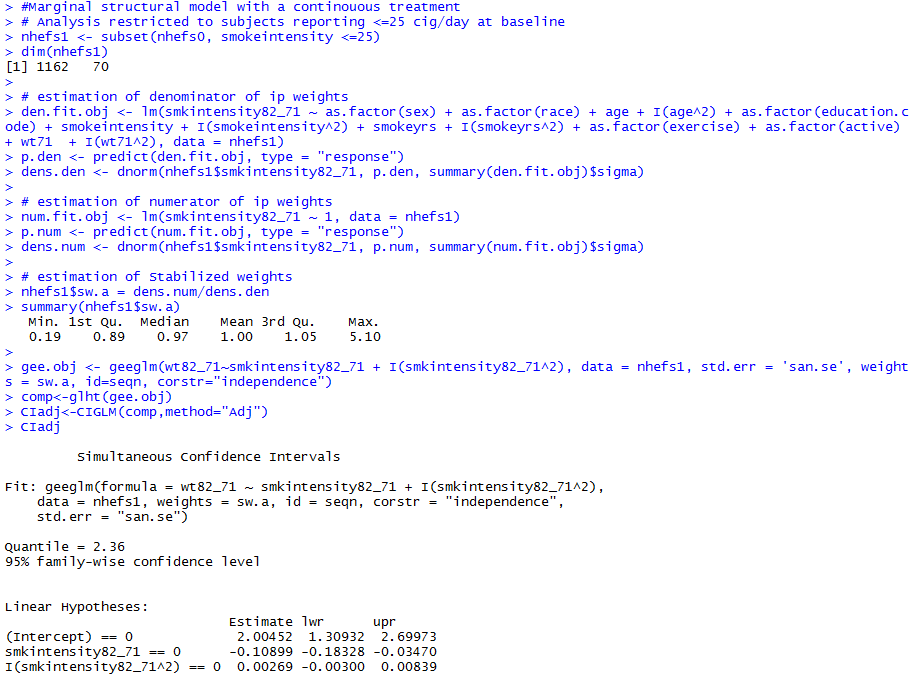
- Change in smoking intensity
- number of cigarettes smoked per day in 1982 minus number of cigarettes smoked per day at baseline
- Nonsaturated model
- For a continuous treatment A, f(A|L) is a probability density function (PDF)
- PDFs are generally hard to estimate correctly
- Using IP weighting for continuous treatments will often be dangerous


Censoring and Missing Data
- We restricted our analyses on 1566 individuals with non-missing data
- may introduce selection bias -
C: indicator for censoring
- C=1 if censored, C=0 if uncensored


- If no selection bias (no arrow from either L or A into C):


Standardization and The Parametric G-Formula
Standardization as an alternative to IP weighting
- The standardized mean outcome in the uncensored treated is a consistent estimator of the mean outcome if everyone had been treated and had remained uncensored
- The standardized mean outcome in the uncensored untreated is a consistent estimator of the mean outcome if everyone had been untreated and had remained uncensored
Under exchangeability and positivity conditional on the variables in L,


We first need to compute the mean outcomes in the uncensored treated in each stratum l of the confounders L


Estimating the Mean Outcome via Modeling
- We fit a linear regression model for the mean weight gain with treatment A and all 9 confounders in L included as covariates
- We can then obtain an estimate
for each combination of values of A and L.


Standardizing the Mean Outcome to the Confounder Distribution
- When all variables in L are discrete, each mean receives a weight equal to the proportion of subjects with values L=l
- The proportions Pr[L=l] could be calculated nonparametrically from the data, but this method becomes tedious for high dimensional data with many confounders
- There is another faster, but mathematically equivalent, method to standardize means
Standardizing the Mean Outcome to the Confounder Distribution


- Create a dataset in which the original data is copied 3 times
- In the second block, set the value of A to 0, and delete the data on the outcome
- In the third block, set the value of A to 1, and delete the data on the outcome
- Fit a regression model for the mean outcome given A and L
- Use the parameter estimates from the model to predict the outcome values for all rows in the second and third blocks
- Compute the average of all predicted values in the second block, which is the standardized mean outcome in the untreated
- The standardized mean outcome in the treated is the average of all predicted values in the third block

Use bootstrap to obtain a 95% confidence interval

IP Weighting vs. Standardization
- IP weighting relies on the correct specification of the treatment model
- Standardization relies on the correct specification of the outcome model
- We should not choose between IP weighting and standardization when both methods can be used to answer a causal question
- Use both methods whenever possible - We can also use doubly robust methods that combine models for treatment and for outcome in the same approach
Summary
- Exchangeability
- Positivity
- Consistency
- No measurement error
- No model misspecification
The validity of causal inferences based on observational data requires the following conditions: