PHC7065 CRITICAL SKILLS IN DATA MANIPULATION FOR POPULATION SCIENCE

Text Data
Hui Hu Ph.D.
Department of Epidemiology
College of Public Health and Health Professions & College of Medicine
March 26, 2018
Introduction to Text Data
Lab: Text Data
Introduction to Text Data
Data types
- Structured data:
- relational databases
- easy to extract information from them
- Semi-structured data:
- loosely formatted XML, JSON
- not challenging to extract information
- Unstructured data
- scholarly literature, clinical notes, research reports, webpages
- majority of data is unstructured
- very challenging to extract information
over 80% of all data
One of the earliest study using Twitter data
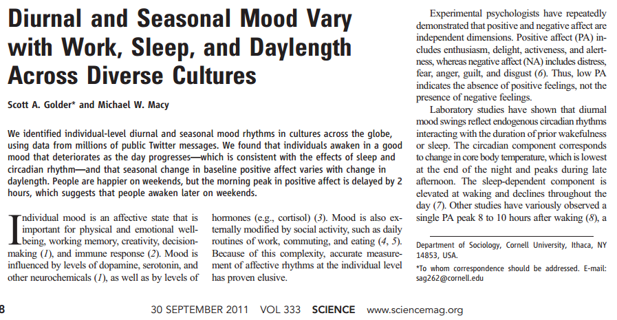
- Examined how trends in positive and negative attitudes varied over the day and the week
- Collected 500 million Tweets produced by more than 2 million people
- Found fascinating daily and weekly trends in attitudes
Tools
- Many tools existed to assist researchers in coding and analyzing dozens or even hundreds of text documents
- However, many of these tools are less useful when the number of documents is in the tens or thousands or millions
- even all researchers in the US work together, they cannot code even the 1% daily sample of Tweets
- We need new tools to collect, categorize, and understand massive text data
- collect and manage the data
- turn the text into numbers of some sort
- analyze the numbers
- Natural Language Processing (NLP): a set of techniques for approaching text problems
Collecting text data
- Querying API
- Twitter API
- Web scraping
- if no API available
- OCR (optical character reader)
- if text record is paper based (e.g. clinical notes)
- Deep learning
- extract house numbers from Google Street View
Turn the text into numbers
- TF-IDF
- NLP Pipeline
- Bag of words
- Word2vec
TF-IDF
- Term frequency-inverse document frequency
- One of the most fundamental techniques for retrieving relevant documents from a corpus
- Can be used to query a corpus by calculating normalized scores that express the relative importance of terms in the documents
- Mathematically expressed as the product of the term frequency and the inverse document frequency:
- tf_idf=tf*idf
- tf: the importance of a term in a specific document
- idf: the importance of a term relative to the entire corpus
TF
- A term's frequency can be simply represented as the number of times it occurs in the text
- more commonly, we normalize it by taking into account the total number of terms in the text, so that overall score accounts for document length relative to a term's frequency
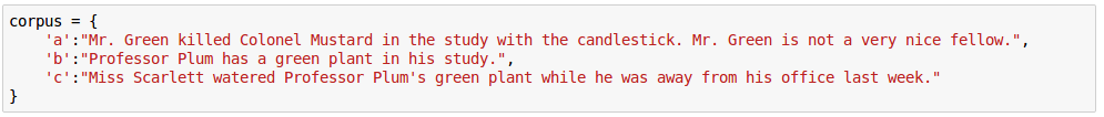
- e.g. "green"
- A common technique for scoring a compound query such as "Mr. Green" is to sum the TF scores for each of the query terms in each document, and return the documents ranked by the summed term frequency score
Limitations of TF
- The term frequency scoring model looks at each document as an unordered collection of words
- queries for "Green Mr." or "Green Mr. Foo" would have returned the exact same scores as the query for "Mr. Green", even though neither of those phrases appears in the sample sentences
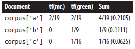
- TF alone does not account for very frequent words, called stopwords, that are common across many documents
- all terms are equally weighted, regardless of their actual importance
- e.g. "the green plant" contains the stopword "the", which skews overall TF scores in favor of corpus['a']
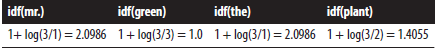
IDF
- A calculation that provides a generic normalization metric for a corpus
- works in general case by accounting for the appearance of common terms across a set of documents by considering the total number of documents in which a query term ever appears
- It produces a higher value if a term is somewhat uncommon across the corpus than if it is common
- helps to account for the problem with stopwords
- "green" returns lower IDF score than "candlestick"
Semantics
- One of the most fundamental weaknesses of TF-IDF is that it inherently does not leverage a deep semantic understanding of the data and throw away a lot of critical context
- Example: let's suppose you are given a document and asked to count the number of sentences in it
- it's a trival task for human
- it's another story entirely for a machine
- Detecting sentences is usually the first step in most NLP pipelines
- it's deceptively easy to overestimate the utility of simple rule-based heuristics
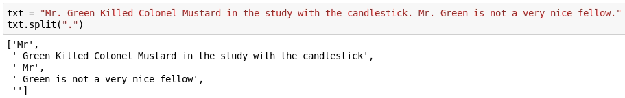
Detecting sentences
- The first attempt at solving the sentence detection problem might be to just count the periods, question marks, and exclamation points in the sentence.
- it is quite crude and has the potential for producing an extremely high margin of error
- Some potential solutions:
- some "Title Case" detection with a regular expression
- construct a list of common abbreviations to parse out the proper noun phrases
NLP Pipeline
- EOS (end-of-sentence) detection
- Tokenization
- POS (part-of-speech) tagging
- Chunking
- Extraction
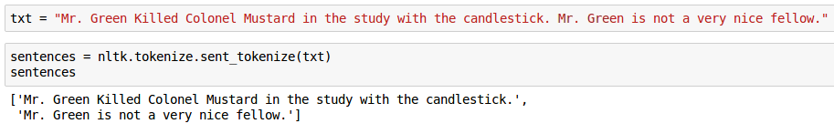
EOS Detection
-
Sentences generally represent logical units of thought, so they tend to have a predictable syntax that lends itself well to further analysis
- This step breaks a text into a collection of meaningful sentences
- most NLP pipelines begin with this step since the next step (tokenization) operates on individual sentences
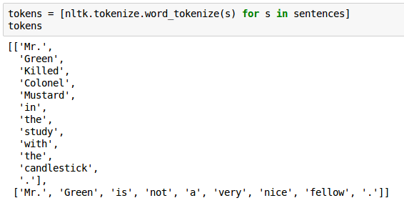
Tokenization
- This step operates on individual sentences, splitting the sentence into tokens
- For this simple example below, tokenization appeared to do the same thing as splitting on whitespace, with the exception that it tokenized out EOS markers correctly, but it can do a bit more
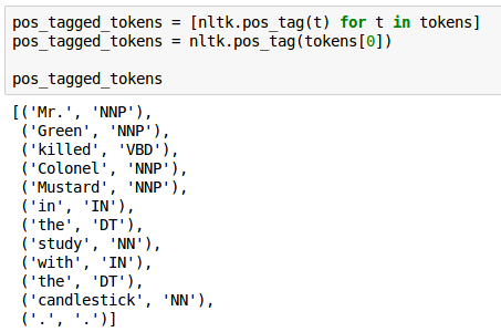
POS tagging
- This step assigns part-of-speech (POS) information to each token
- by using these POS tags, we will be able to chunk together nouns as part of noun phrases and then try to reason about what types of entities they might be (e.g. people, places, or organizations)
noun
verb
Chunking and Extraction
- Chunking involves analyzing each tagged token within a sentence and assembling compound tokens that express logical concepts
- Extraction involves analyzing each chunk and further tagging the chunks as named entities, such as people, organizations, locations, etc.

Bag of Words
- The Bag of Words model learns a vocabulary from all of the documents, then models each document by counting the number of times each word appears
- Example:
- sentence 1: "The cat sat on the hat"
- sentence 2: "The dog ate the cat and the hat"
- Our vocabulary is:
{the, cat, sat, on, hat, dog, ate, and}
- We count the number of times each word occurs in each sentence to get our bag of words:
- sentence 1: {2,1,1,1,1,0,0,0}
- sentence 2: {3,1,0,0,1,1,1,1}
Word2vec
- A neural network implementation that learns distributed representations for words
- published by Google in 2013: Mikolov T, Chen K, Corrado G, Dean J. Efficient estimation of word representations in vector space. arXiv preprint arXiv:1301.3781. 2013 Jan 16.
- Word2vec does not need labels in order to create meaningful representations
- very useful since most data in the real word is unlabeled
- Words with similar meanings appear in clusters, and clusters are spaced such that some word relationships such as analogies can be reproduced using vector math
- example: king - man + woman = queen
- Distributed word vectors are powerful and can be used for many applications, particularly word prediction and translation
From Words to Paragraphs
- The lengths of text data are usually different in different documents
- e.g. variable-length movie reviews
- we need to find a way to take individual word vectors and transform them into a feature set that is the same length for every review
- Methods:
- vector averaging: simply average the word vectors in a given document
- clustering: using clustering algorithm such as K-Means to assign a cluster (centroid) for each word, and then define a function to convert documents into bags-of-centroids
- these two methods have similar performance as bag of words, since none of them preserves word order information
- A better method: paragraph vector (Doc2vec)