建國中學
暑假地球科學讀書會
大氣動力學
Presenter: 122527 Brine
Index
Forces
- pressure gradient force, PGF
- gravitational force
- viscosity
- friction
apparent Forces
- aka pseudo force
- centrifugal force
- coriolis force
whiteboard time
Drawing on computer is hard. Have mercy on me.
Pressure gradient force
- assume there's an air parcel
a_x = -\frac{1}{\rho}\frac{\partial P}{\partial x\ }
a_y = -\frac{1}{\rho}\frac{\partial P}{\partial y\ }
a_z = -\frac{1}{\rho}\frac{\partial P}{\partial z\ }
Gravitational force
\vec{F_g} = \frac{GMm}{r^2}(\frac{\vec r}{r})
\frac{\vec{F_g}}{m} = \frac{GM}{r^2}(\frac{\vec r}{r}) \equiv \vec {g^*}
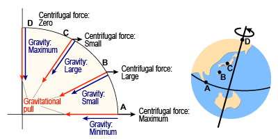
Centrifugal Force
\vec g = \vec{g^*} + \Omega^2 \vec R
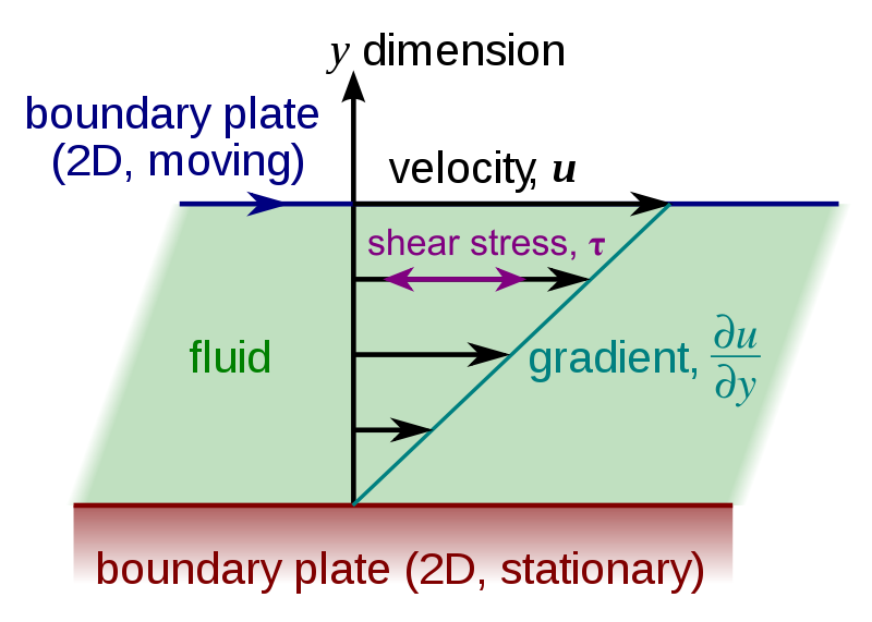
Viscosity
x is parallel to the line of latitude
y is parallel to the line of longitude
z is the altitude
\dot x \leftrightarrow u \\
\dot y \leftrightarrow v \\
\dot z \leftrightarrow w
F = \mu A \frac{\Delta u}{\Delta z}
(observed)
\tau_{z \to x} = \large \frac{F}{A} \normalsize = \mu \large \frac{\partial u}{\partial z}
Viscosity
a_{z \to x} = \frac{(\tau_u - \tau_d)\Delta zA \\}{m}
\\ = \frac{\frac{\partial}{\partial z} \tau_{z \to x} \Delta x \Delta y \Delta z}{m}
\\ = \frac{1}{\rho} \frac{\partial}{\partial z} \tau_{z \to x}
\\ = \frac{\mu}{\rho} \frac{\partial}{\partial z} \frac{\partial u}{\partial z}
\\ = \nu \frac{\partial^2 u}{\partial z^2}
a_x = a_{x \to x} + a_{y \to x} + a_{z \to x}
= \nu [\frac{\partial^2 u}{\partial x^2} + \frac{\partial^2 u}{\partial y^2} + \frac{\partial^2 u}{\partial z^2}]
= \nu \nabla^2 u
\nabla = \displaystyle
\sum_{i=1}^n \vec e_i {\partial \over \partial x_i} = \left({\partial \over \partial x_1}, \ldots, {\partial \over \partial x_n} \right)
coriolis force
Using simple calculus
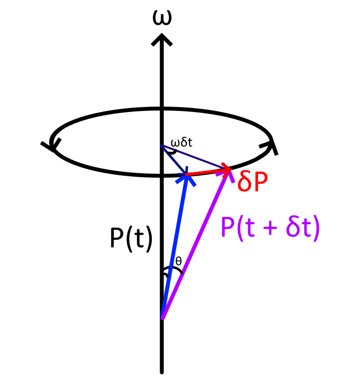
\delta P \approx P\sin\theta\omega\delta t
\frac{DP}{Dt} = \omega \times P + \frac{dP}{dt}
\frac{Dr}{Dt} = \omega \times r + \frac{dr}{dt}
\frac{D^2r}{Dt^2} = \omega \times \frac{Dr}{Dt} + \frac{Dv}{Dt}
coriolis force
Using simple calculus
coriolis force
Using simple calculus
\frac{Dr}{Dt} = \omega \times r + v
\frac{D^2r}{Dt^2} = \omega \times \frac{Dr}{Dt} + \frac{Dv}{Dt}
\frac{DP}{Dt} = \omega \times P + \frac{dP}{dt}
\frac{D^2r}{Dt^2} = \omega \times (\omega \times r + v) + \omega \times v + \frac{dv}{dt}
A = \frac{dv}{dt} + 2 \omega \times v + \omega^2r
coriolis force
Another approach - u
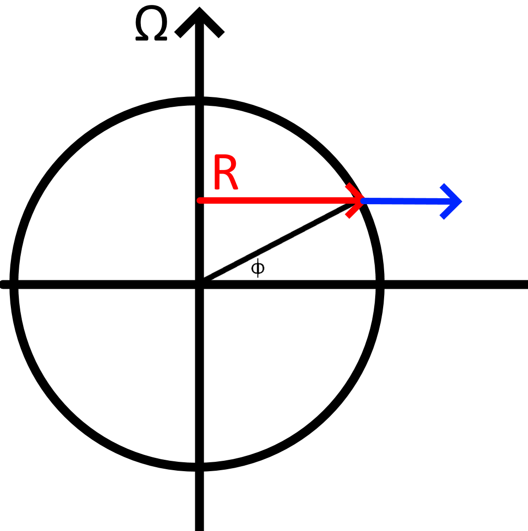
(\Omega + \frac{u}{R})^2 \vec{R}
= \Omega^2 \vec{R} + 2\Omega u \frac{\vec R}{R} + (\frac{u}{R})^2 \vec R
2 \Omega u \cos \phi
-2 \Omega u \sin \phi
coriolis force
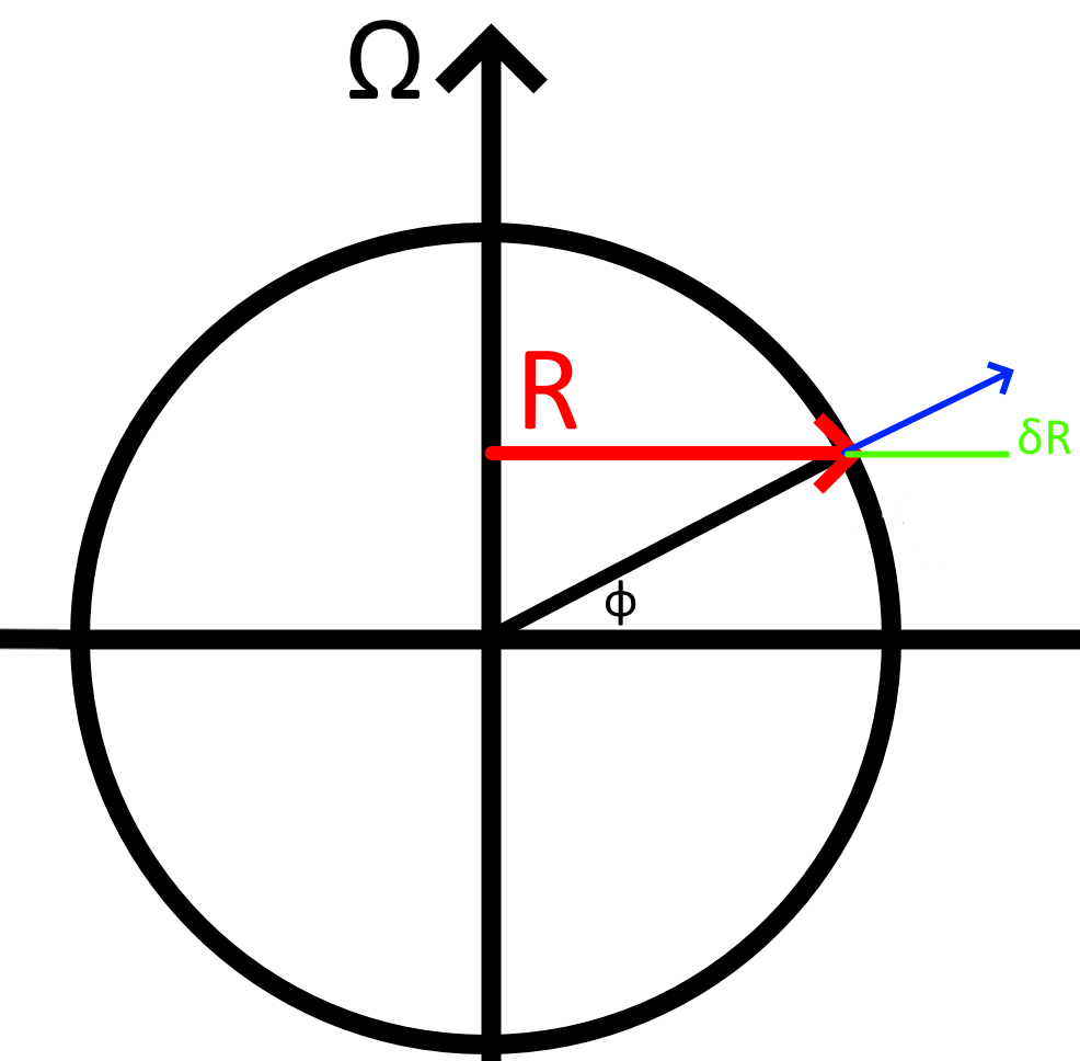
Another approach - v
conservation\ of\ angular\ momentum
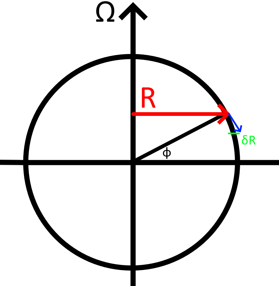
\Omega R^2 = (\Omega + \frac{\delta u}{R + \delta R})(R + \delta R)^2
\delta u \approx -2\Omega\delta R
\delta R = \delta y \sin \phi
\frac{du}{dt} = 2\Omega v \sin \phi
coriolis force
Another approach - w
conservation\ of\ angular\ momentum
\Omega R^2 = (\Omega + \frac{\delta u}{R + \delta R})(R + \delta R)^2
\delta u \approx -2\Omega\delta R
\delta R = \delta z \cos \phi
\frac{du}{dt} = -2\Omega w \cos \phi
coriolis force
Another approach - conclusion
\Biggl \{
\frac{d\vec V}{dt}
\Large\frac{du}{dt}\normalsize = 2\Omega v \sin \phi - 2 \Omega w \cos \phi
\Large\frac{dv}{dt}\normalsize = - 2 \Omega u \sin \phi
\Large\frac{dw}{dt}\normalsize = 2 \Omega u \cos \phi
coriolis force
Another approach - conclusion
\Biggl \{
\frac{d\vec V}{dt}
\Large\frac{du}{dt}\normalsize = 2\Omega v \sin \phi - 2 \Omega w \cos \phi
\Large\frac{dv}{dt}\normalsize = - 2 \Omega u \sin \phi
\Large\frac{dw}{dt}\normalsize = 2 \Omega u \cos \phi
f \equiv 2 \Omega\sin\phi
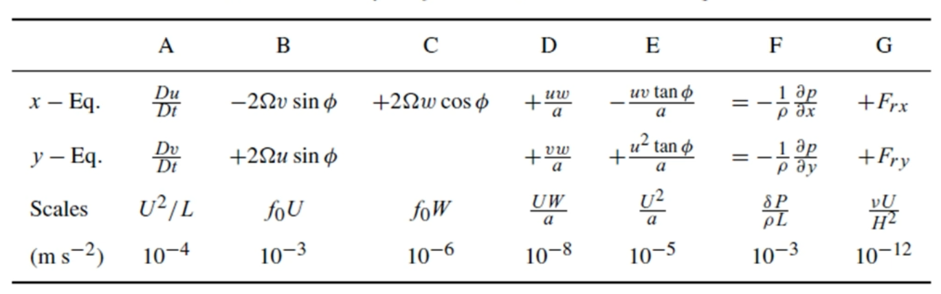
Equations
Introduction to some of the equations
Motion equatoins
\frac{d \vec V}{dt} = \vec g - \frac{1}{\rho} \nabla P + \nu \nabla^2 \vec V - 2 \vec \Omega \times \vec V
-2\vec \Omega \times \vec V = -2\Omega \begin{vmatrix}
\hat i & \hat j & \hat k\\
0 & \cos \phi & \sin \phi\\
u & v & w
\end{vmatrix}
spherical coordinate system
(x, y, z) \rightarrow (\theta( sometimes\ \lambda), \phi, r)
\Biggl \{
dx = r \cos \phi d\theta
dy = rd\phi
dz = dr
\vec V = (u, v, w) = \hat i u + \hat j v + \hat k w
spherical coordinate system
\frac{d(\hat i u)}{dt} = \hat i \frac{du}{dt} + u \frac{d\hat i}{dt}
spherical coordinate system
\frac{d(\hat i u)}{dt} = \hat i \frac{du}{dt} + u \frac{d\hat i}{dt}
\frac{d\hat i}{dt} = \frac{\partial \hat i}{\partial t} + u \frac{\partial \hat i}{\partial x}
\Large|\frac{\partial \hat i}{\partial x}| \normalsize= \displaystyle \lim_{\delta x \to 0} \frac{|\delta i|}{\delta x}
= \frac{|\hat i|\delta \theta}{r \cos \phi \delta \theta} = \frac{1}{r\cos \phi}
\delta \hat i = \sin \phi \hat j - \cos \phi \hat k
\delta \hat i
\sin \phi \hat j
- \cos \phi \hat k
spherical coordinate system
\frac{d(\hat i u)}{dt} = \hat i \frac{du}{dt} + u \frac{d\hat i}{dt}
\frac{d\hat i}{dt} = \frac{\partial \hat i}{\partial t} + u \frac{\partial \hat i}{\partial x}
\Large|\frac{\partial \hat i}{\partial x}| \normalsize= \displaystyle \lim_{\delta x \to 0} \frac{|\delta i|}{\delta x}
= \frac{|\hat i|\delta \theta}{r \cos \phi \delta \theta} = \frac{1}{r\cos \phi}
u \frac{d\hat i}{dt} = u^2 \frac{\partial \hat i}{\partial x} = \frac{u^2}{r} \tan \phi \hat j - \frac{u^2}{r} \hat k
\frac{D\vec V_y}{Dt} = (\frac{Du}{Dt} + \frac{u^2}{r} \tan \phi + \frac{vw}{r}) \hat j
= - \frac{1}{\rho}\frac{\partial P}{\partial y} - 2\Omega u \sin\phi + F_y
\delta \hat i = \sin \phi \hat j - \cos \phi \hat k
\delta \hat i
\sin \phi \hat j
- \cos \phi \hat k
HORIZONTAL Approximation
geostrophic\ wind
-fv \approx -\frac{1}{\rho}\frac{\partial P}{\partial x} \rightarrow v \approx \frac{1}{f\rho}\frac{\partial P}{\partial x}
fu \approx -\frac{1}{\rho}\frac{\partial P}{\partial x} \rightarrow u \approx \frac{1}{f\rho}\frac{\partial P}{\partial y}
HORIZONTAL Approximation
geostrophic\ wind
-fv \approx -\frac{1}{\rho}\frac{\partial P}{\partial x} \rightarrow v \approx \frac{1}{f\rho}\frac{\partial P}{\partial x}
fu \approx -\frac{1}{\rho}\frac{\partial P}{\partial x} \rightarrow u \approx \frac{1}{f\rho}\frac{\partial P}{\partial y}
\frac{Du}{Dt} \approx - \frac{1}{\rho}\frac{\partial P}{\partial y} - \small{2\Omega u \sin\phi}
= - f(u - u_g)
= - \frac{1}{\rho}\frac{\partial P}{\partial y} - \small{2\Omega u \sin\phi} + F_y
\longrightarrow
(\frac{Du}{Dt} + \frac{u^2}{r} \small{\tan \phi} + \frac{vw}{r}) \hat j
Rossby number
- a tool to see whether the approximation is valid
Ro = \frac{a_{total}}{a_{coriolis}} = \frac{\frac{Du}{Dt}}{fu} = \frac{u / (l / u)}{fu} = \frac{u}{fl}
Ro < \frac{1}{10} \leftrightarrow valid
VERTICAL Approximation
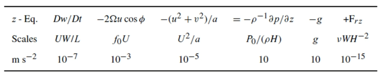
\frac{dw}{dt} = - g - \frac{1}{\rho}\frac{\partial P}{\partial z}
\rightarrow
\frac{dw}{dt} \approx 0 \leftrightarrow equilibrium
tiny turbulence
g \approx - \frac{1}{\rho_0}\frac{\partial P_0}{\partial z}
P = P_0(z) + P'(x,y,z,t)
\rho = \rho_0(z) + \rho'(x,y,z,t)
\frac{dw}{dt} = - g - \frac{1}{\rho_0 + \rho'}\frac{\partial(P_0 + P')}{\partial z}
\forall \small x\ s.t.\ 0 < x << 1,\ \frac{1}{1 + x} \approx 1 - x
\frac{dw}{dt} \approx - \frac{1}{\rho_0}\frac{\partial P'}{\partial z} - \frac{\rho'}{\rho_0}g
continuity equation
x_{in} - x_{out} = - (\frac{\partial}{\partial x}\delta x) \rho u \delta y\delta z
...
- (\frac{\partial}{\partial x} \rho u + \frac{\partial}{\partial y} \rho v + \frac{\partial}{\partial z} \rho w)\delta x\delta y\delta z
= \frac{\partial \rho}{\partial t} \delta x\delta y\delta z
\frac{\partial \rho}{\partial t} +\small \nabla \cdot (\rho\vec V) = 0 \leftrightarrow \frac{D\rho}{Dt}+ \small \rho \nabla\cdot \vec V = 0
\nabla \cdot \vec v = \frac{\partial v_x}{\partial x} + \frac{\partial v_y}{\partial y} +\frac{\partial v_z}{\partial z}...
another way
M = \rho V
\frac{DM}{Dt} = 0
\frac{1}{M}\frac{D}{Dt}\small(\rho V) = 0
\frac{1}{\rho}\frac{D\rho}{Dt}+ \frac{1}{V}\frac{DV}{Dt}\small = 0
\frac{1}{\rho}\frac{D\rho}{Dt}+ \small \nabla\cdot \vec V = 0
(\frac{\partial }{\partial x} xyz = yz)\\
(\frac{\partial x}{\partial t}yz + \frac{\partial y}{\partial t}xz + \frac{\partial y}{\partial t}xz = \frac{DV}{Dt})
a bit of Manoeuvre
\frac{1}{\rho}\frac{D\rho}{Dt}+ \small \nabla\cdot \vec V = 0
\rho = \rho_0(z) + \rho'(x,y,z,t)
\frac{1}{\rho_0+\rho'}\frac{D(\rho_0+\rho')}{Dt} + \nabla \cdot \vec V = 0
\large\frac{1}{\rho_0}\normalsize(\frac{\partial \rho'}{\partial t} + \small\vec V \cdot \nabla \rho') + \large\frac{1}{\rho_0}\frac{dz}{dt}\frac{d\rho_0}{dz} + \small\nabla \cdot \vec V \approx 0
\large\frac{1}{\rho_0}\normalsize w\frac{d\rho_0}{dz} + \small\nabla \cdot \vec V \approx 0
\frac{d\rho_0}{dz}w + \rho_0\small\nabla \cdot \vec V \approx 0
\frac{\partial\rho_0}{\partial x}u +\frac{\partial\rho_0}{\partial y}v +\frac{\partial \rho_0}{\partial z}w +
\rho_0 \frac{\partial u}{\partial x}+\rho_0 \frac{\partial v}{\partial y}+\rho_0 \frac{\partial w}{\partial z}+
\approx 0
\nabla \cdot (\rho_0 \vec V)
\approx 0
How similar
\nabla \cdot (\rho_0 \vec V)
\approx 0
incompressible\ flow
\frac{1}{\rho}\frac{D\rho}{Dt}+ \small \nabla\cdot \vec V = 0
\delta \rho = 0
\small \nabla\cdot \vec V = 0
\small \nabla\cdot (\rho \vec V) = 0
\frac{d\rho_0}{dz}w + \rho_0\small\nabla \cdot \vec V \approx 0
Application
What can we do with all of that
Weather forecasting
of course- many models use the equations mentioned above
- prediction for weather / climate
what if
- predict what the world will look like with different conditions
thank you
I've got nothing left lmao