Basics of
Earth Observation and Remote Sensing


Britta Ricker, PhD
Objectives of this assignment
Use the basic functionalities of remote sensing for spatial data processing;
- Measure land cover change overtime;
-
Visualize the results
Today in Class
- GIS & Remote Sensing
- Color Composites
- Vegetation Indices
- CyberGIS and Big Data
- Review: How do these concepts relate to land use change?


Disaster and Land Use


Online "slippy" maps

Maps can help reduce complexity


Vanacker (2016) Impact of deforestation on slope stability

McSweeney (2017) Cocaine trafficking is destroying Central Americ's forests
Geographic Information
Science
Geographic Information Systems(GIS)

Geographic Information Systems (GIS)

Remote Sensing

Remote Sensing

Lidar


1 m resolution!
Remote Sensing
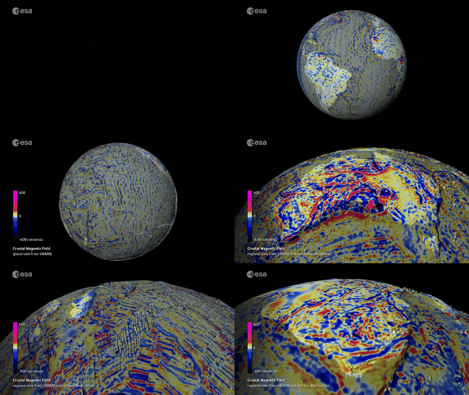
Remote Sensing
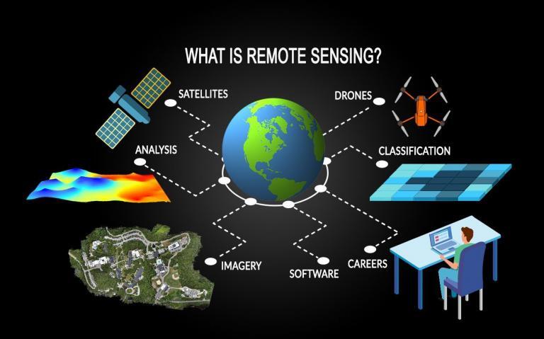
Remote Sensing

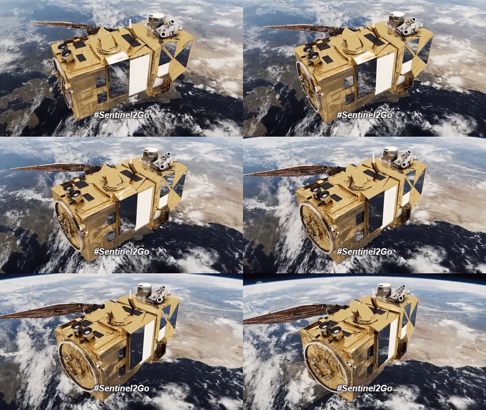
Temporal Resolution: Revisit Every 5 days
True Color

Details
From Sentinel 2
Date of image: 22 Feb 2017
Spatial Resolution:
Each pixel represents 20 m
2325 columns
2960 rows of pixels

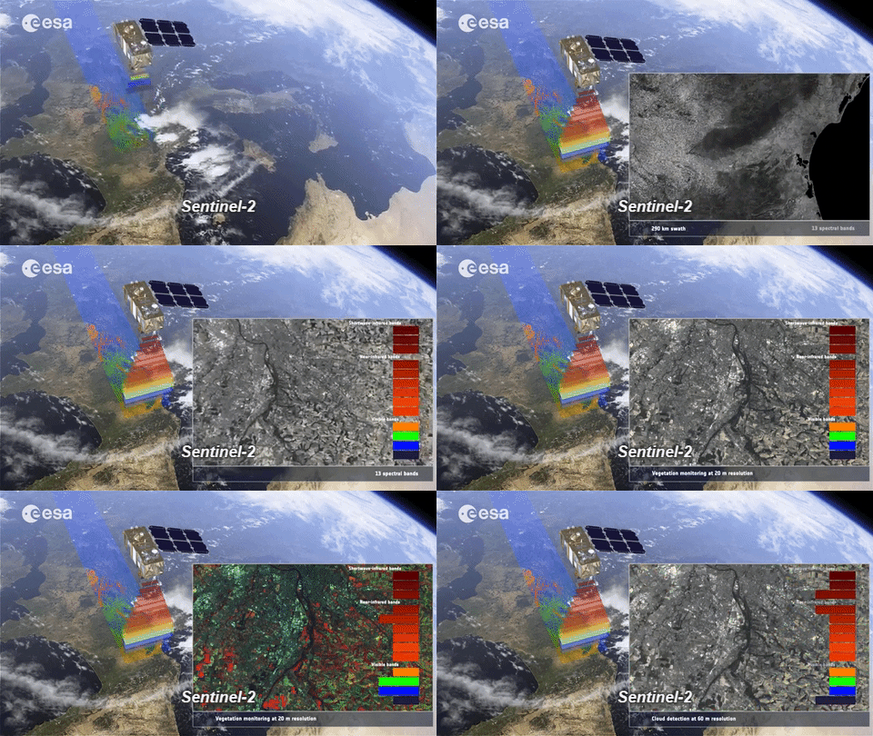
Sentinel 2
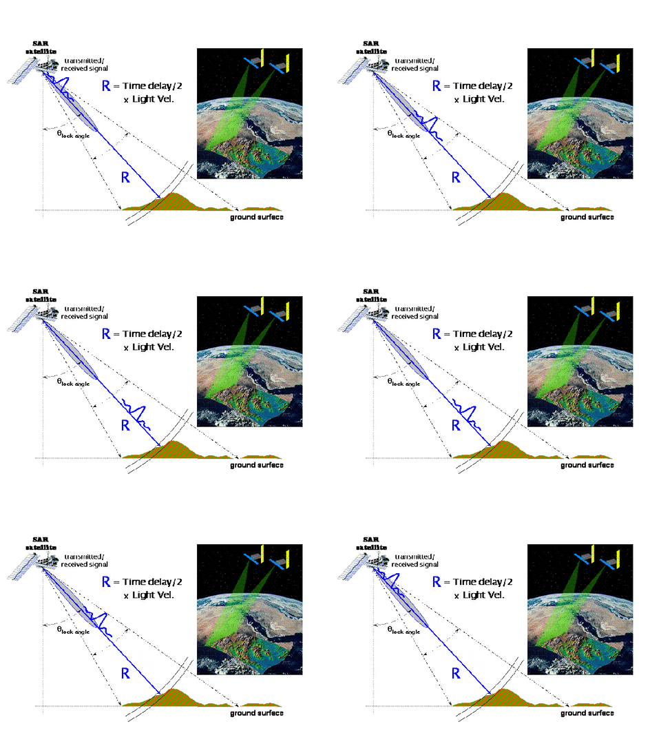
Active Sensor
Passive Sensor

Electromagnetic Energy
Features on the Earth reflect, absorb, transmit, and emit electromagnetic energy from the sun.

Properties of electromagnetic energy
Multispectral imagery
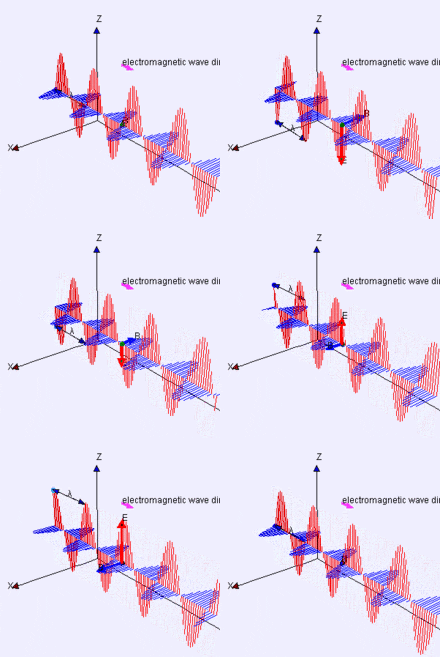
wavelength, fequency, amplitude

The visible spectrum is small!

What else is collected?
Bands and spectral ranges

Spectral signature

How are images rendered on our screen?
3 bands projected light
The primary colors are Red, Green, Blue
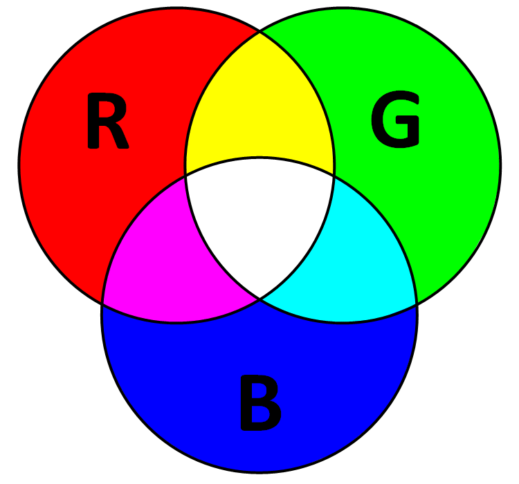
True Color
= Band 4 Red
= Band 3 Green
= Band 2 Blue

False Color Composites

Urban areas

Urban=Purple
= Band 12 SWIR II
= Band 11 SWIR I
= Band 4 Red
Vegetation
= Band 8 NIR
= Band 4 Blue
= Band 3 Red

Spectral signature
Bands and spectral signatures


What Are Vegetation Indices?

Healthy vegetation


Normalized Difference Vegetation Index
NDVI=NIR-IR/NIR+IR
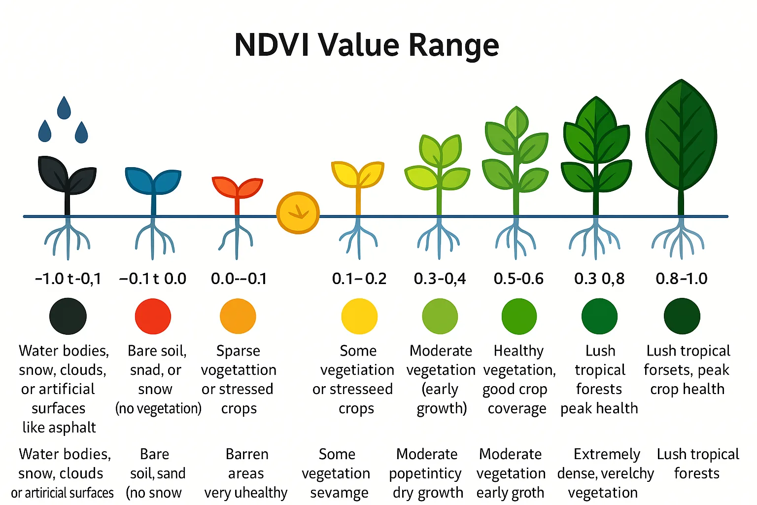
Interpreting NDVI Values
Values range from -1 to +1; higher values indicate healthier vegetation.

Applications of NDVI
- Agriculture monitoring
- Forest health assessment
- Climate change studies

Interpreting NDVI Values
Values range from -1 to +1; higher values indicate healthier vegetation.
Animation
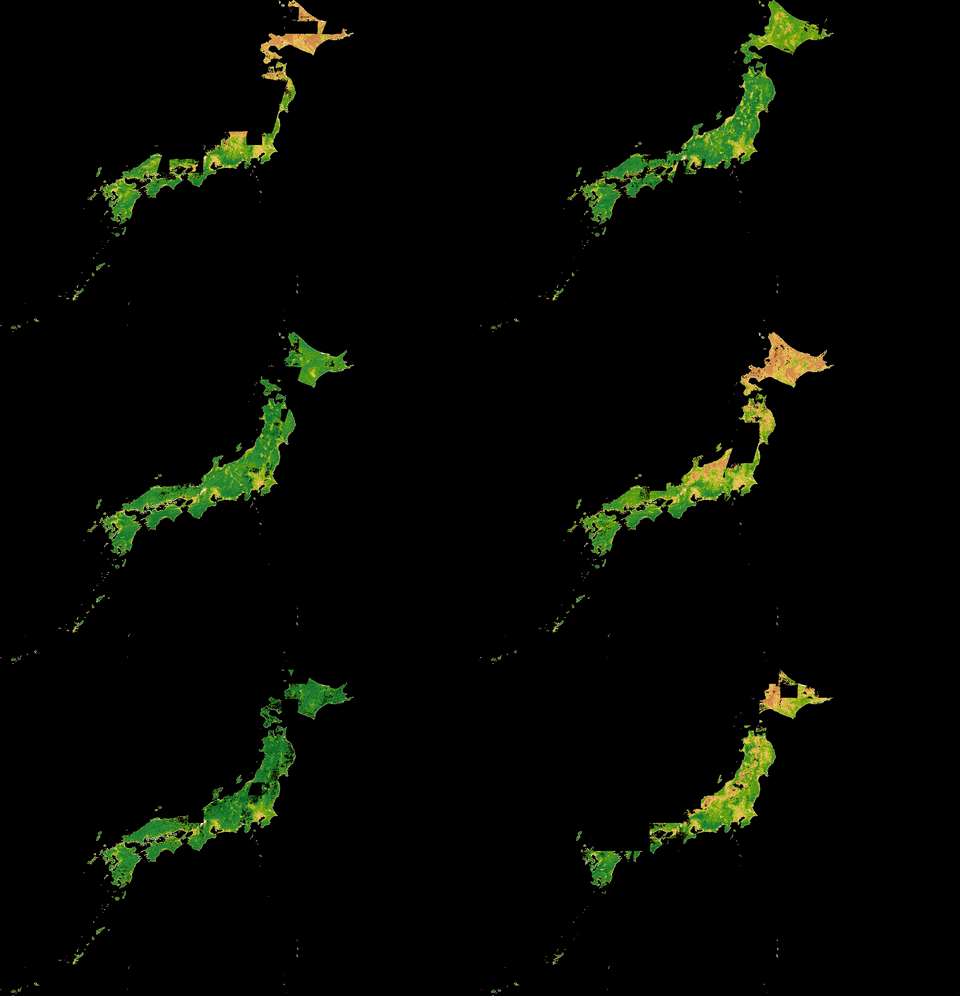
What is happening?
Japan Monthly NDVI 2023-2024
https://code.earthengine.google.com/2ae81299e3974222111d44df7c85e1e1
Assignment today
Tomorrow: Classification
Supervised & Unsupervised

Big Data and
CyberGIS
Cloud Computing



-
valuable for information dissemination
-
faster and more data processing that was not previously possible
-
data access
Google Earth Engine
-
Cloud-based platform for geospatial analysis
-
Access over 40 years of satellite imagery
-
Upload own data sets to integrate with publicly available data
-
Apply range of common algorithms to data
-
Export images, tables, charts, map outputs


Hansen et al (2013)
High-Resolution Global Maps of 21st-Century Forest Cover Change, Science
15 Nov. Vol. 342, Issue 6160, pp. 850-853 DOI: 10.1126/science.1244693.
What does this code do?
// Load Sentinel-2 TOA reflectance data.
var dataset = ee.ImageCollection('COPERNICUS/S2_HARMONIZED')
                  .filterDate('25-01-01', '2025-12-30')
                  // Pre-filter to get less cloudy granules.
                  .filter(ee.Filter.lt('CLOUDY_PIXEL_PERCENTAGE', 20))


//true color
var rgbVis = {
  min: 0.0,
  max: 2500,
  bands: ['B4', 'B3', 'B2'],
};
//urban visualization
var urbanVis = {
  min: 0.0,
  max: 2500,
  bands: ['B12', 'B11', 'B4'],
};

//Agriculture visualization
var agVis = {
  min: 0.0,
  max: 2500,
  bands: ['B11', 'B8', 'B2'],
};
//Healthy vegitation visualization
var VegVis = {
  min: 0.0,
  max: 2500,
  bands: ['B8', 'B11', 'B2'],
};

//Land Water visualization
var WaterVis = {
  min: 0.0,
  max: 2500,
  bands: ['B8', 'B11', 'B4'],
};

//Utrecht
Map.setCenter(5.104480, 52.092876, 11);

//different layers
Map.addLayer(dataset.median(), rgbVis, 'RGB');
Map.addLayer(dataset.median(), urbanVis, 'Urban');
Map.addLayer(dataset.median(), agVis, 'Agriculture');
Map.addLayer(dataset.median(), VegVis, 'Vegitation');
Map.addLayer(dataset.median(), WaterVis, 'Water');

//END
//first you will need to use the drawing tools in Google Earth Engine to draw the geometry of the bounding box of your area of interest - the rest of the script should work after that. To see a fully working version - use the script with the geography baked in
//Call the Sentinel 2 dataset and change the date based on the range that interest you - this will create a cloudless mosaic from pixels within that date range.
var S2_collection = ee.ImageCollection('COPERNICUS/S2_HARMONIZED')
.filterBounds(geometry)
.filterDate('2025-07-01', '2025-12-31')
.filterMetadata('CLOUDY_PIXEL_PERCENTAGE', 'less_than', 5)
;
//here create a mosaic with the median value of each pixel within the date range specified and clip to the region I identified in the bounding box called geometry
var S2_mosaic = S2_collection.median().clip(geometry);
// Next call bands B4 as red B3 as green and B2 as blue to make a true color composite to generate in the results Sentinel-2
var S2_display = {bands: ['B4', 'B3', 'B2'], min: 0, max: 3000};
//Add this layer to the map and name the layer true color - you can change the name if you want
Map.addLayer(S2_mosaic, S2_display, "True Color");
//center the map on the bounding box
Map.centerObject(geometry);
//Export image - set the scale based on the bounding box size - I have it set on Aruba
Export.image.toDrive({
image: S2_mosaic,
region: geometry,
description: 'S2_ROI_07-12-2025',
scale: 30,
})
Text
Getting started in Google Earth Engine
Cut and paste this code
Draw bounding box
Summary
Benefits of CyberGIS
- Data access
- Distributed data processing for analysis in the cloud
- Information dissemination through interactive visualizations
Review!
In your own words...
What is the difference between an active and passive sensor?
What is a spectral signature?
What is a false-color composite?
How are they useful for land use change monitoring?
Spatial and
temporal resolution
What do these terms mean and how are they different?

Name two strengths of CyberGIS and cloud computing?
Name two different web cartography Visualization techniques to show change over time.
Thank you!
