Bayesian inversion of 3D groundwater flow
within the Sydney-Gunnedah-Bowen Basin

@BenRMather @MullerDietmar @TheCraigONeill @adambeallgeo @wv2017 @LouisMoresi
Ben Mather, Dietmar Muller, Craig O'Neill, Adam Beall, Willem Vervoort, Louis Moresi

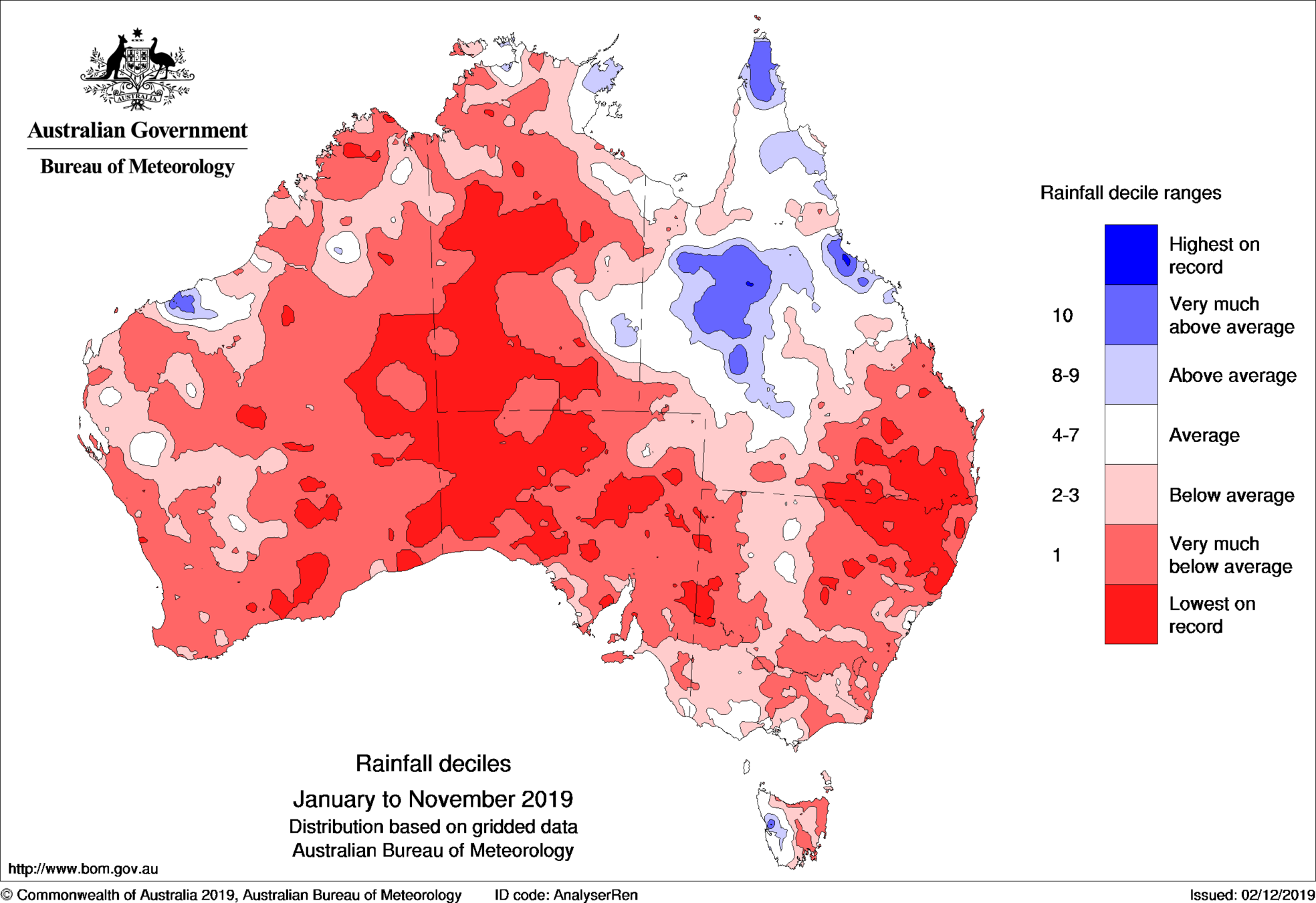
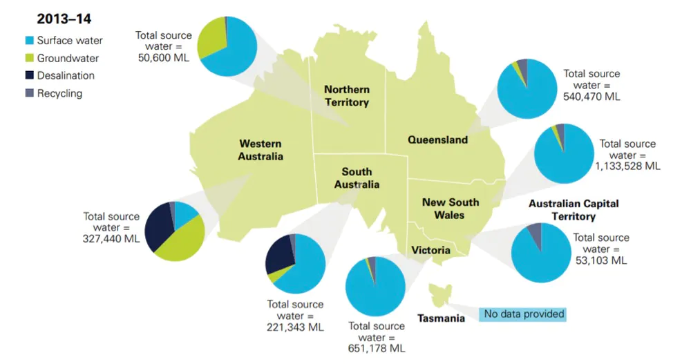
The driest inhabited continent

Australian population
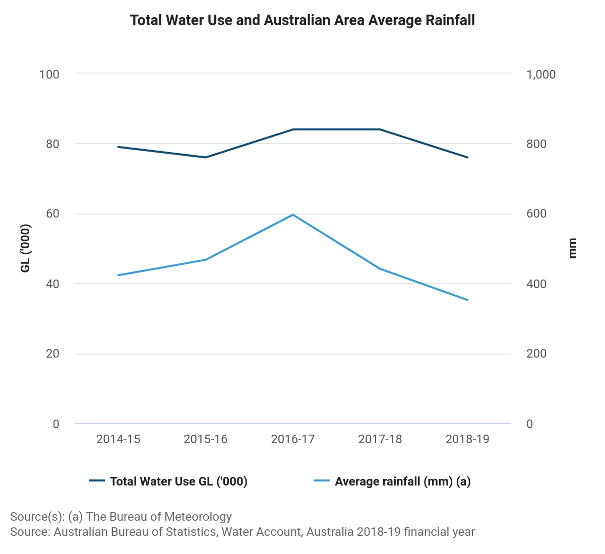
Squeeze on surface water
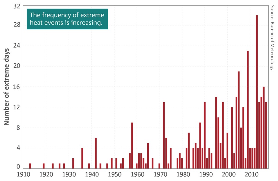
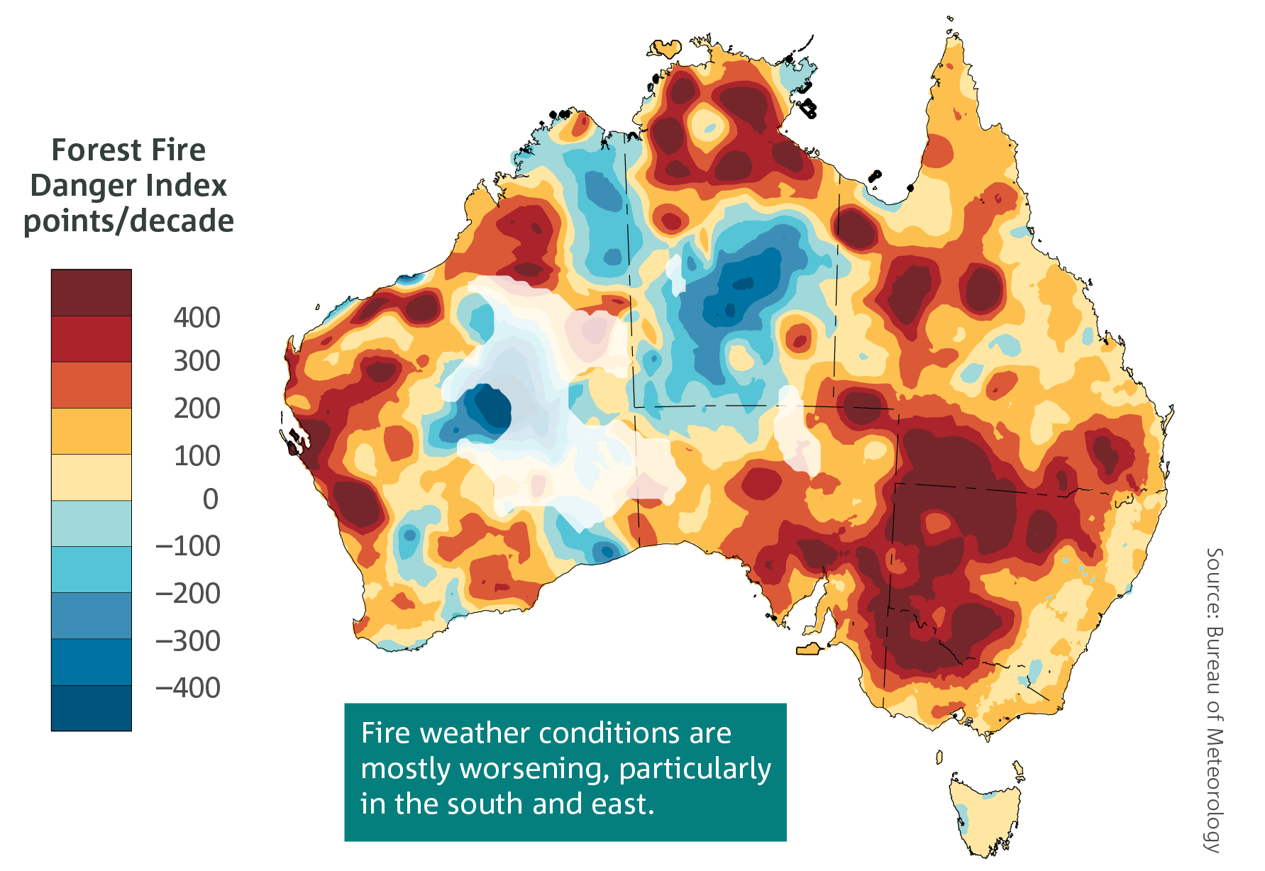
Surface water reserves have become increasingly stretched. With longer droughts, more bushfire days and a growing population, we must seek alternate sources of water.
Groundwater resources
Much is unknown about the dynamics of groundwater flow in Australia, including:
- How geology affects local to regional flow patterns
- Timescales of groundwater flow through major aquifers
- Hydraulic pressure within different layers
- Whether saltwater intrusion affects coastal aquifers
Understanding these factors can help us better manage Australia's groundwater resources.
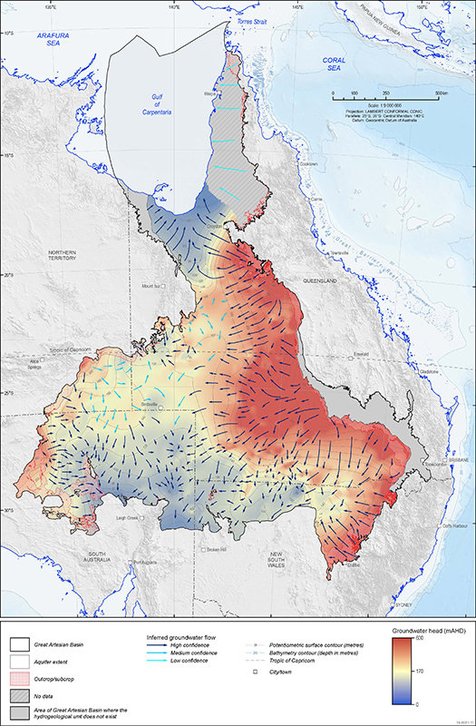
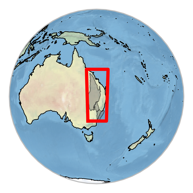
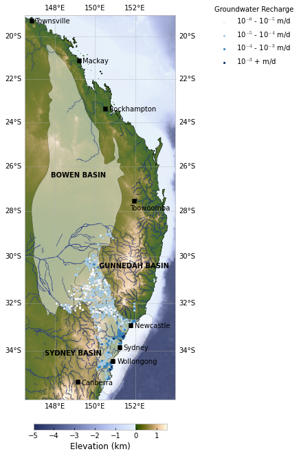
Great Artesian Basin - GA
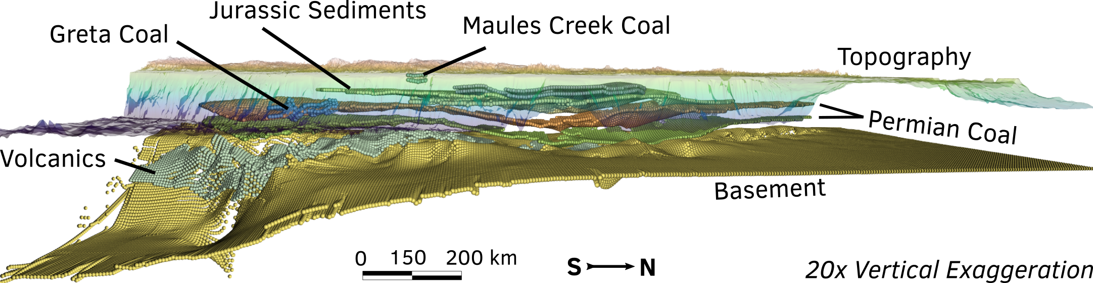
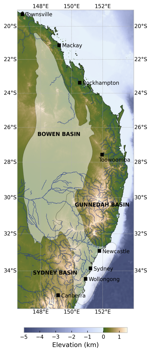
Coupled groundwater-thermal numerical models of the
Sydney-Gunnedah-Bowen Basin
We have:
- Temperature gradients measured in boreholes
- Recharge estimates from Cl mass balance
- Hydraulic pressure measured in wells
- 3D geological model of the basin
We want:
- Groundwater flow velocities within major aquifers
- Capacity of aquifers to store groundwater
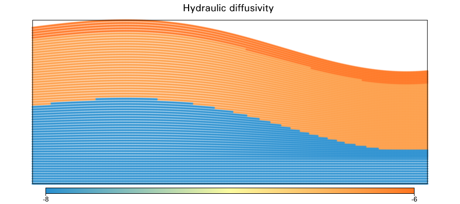
Numerical model - coupling heat flow and fluid flow
Advection-diffusion equation:
Coupling fluid flow with heat flow:
- Solve steady-state Darcy flow to find q
- Substitute q into advection-diffusion equation to solve heat equation.
- Repeat step 2 until convergence is reached.
Implemented using Underworld 2
hydraulic = blue
thermal = red
lower BC
upper BC
side BC
Bayes' Theorem
- Formally describes the link between observations, model, & prior information.
- Where these intersect is called the posterior
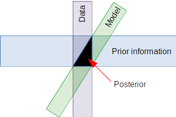
posterior
likelihood
prior
model
data
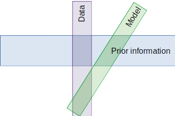
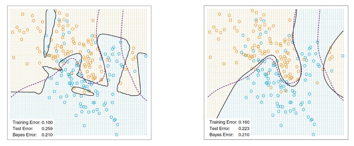
example of an ill-posed problem
example of a well-posed problem
Data-driven
- Use the data to "drive" the parameter exploration.
- Infer what input parameters you need to satisfy your data and prior information
Input parameters
Model being solved
Compare data & priors
FORWARD MODEL
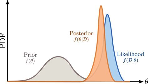
Prior
Likelihood
Posterior
REPEAT
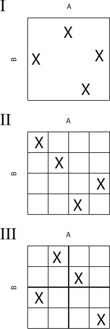
Sampling the posterior
The posterior must be properly sampled to avoid local minima e.g. MCMC, Newton method, etc.

Misfit
Global
minimum
Local
maximum
Local
minimum
A "misfit" function is chosen to find the minimum misfit between data and priors.
Sample the posterior - more!
Misfit
Global
minimum
Local
maximum
Local
minimum
More thoroughly sampling the posterior will identify local min and max
We initialise a MCMC "random walk" at multiple starting points generated from a Latin Hypercube to ensure we are not trapped by local minima.
After N samples the topology of is understood and gradient-optimisation is employed to quickly descend to
Random Sampling
Latin Hypercube
Non-uniqueness
There may be many solutions that fit the same set of observations.

Data Assimilation
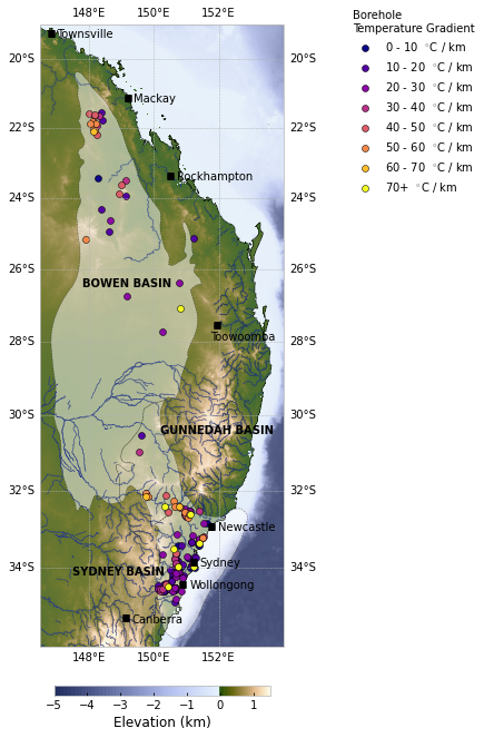
3) Temperature gradients
1) Chloride concentration
2) Hydraulic Pressure Head
Data Assimilation
1) Chloride concentration
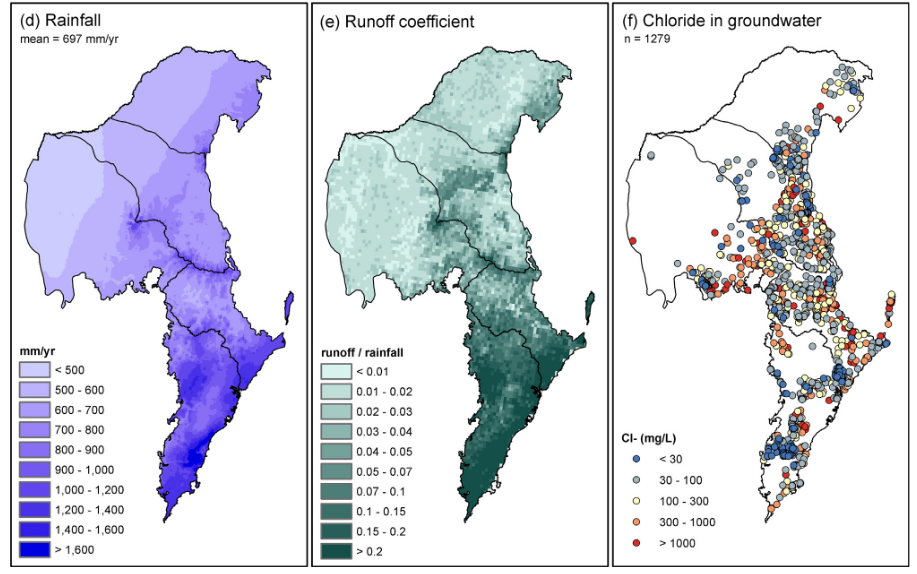
Chloride is excluded from evapotranspiration and leaches downward into the water table to become a proxy for recharge.
Chloride concentration of rainfall
Chloride concentration of groundwater
mean annual rainfall
Crosbie et al. 2018
Data Assimilation
1) Chloride concentration
3) Temperature gradients
2) Hydraulic Pressure Head
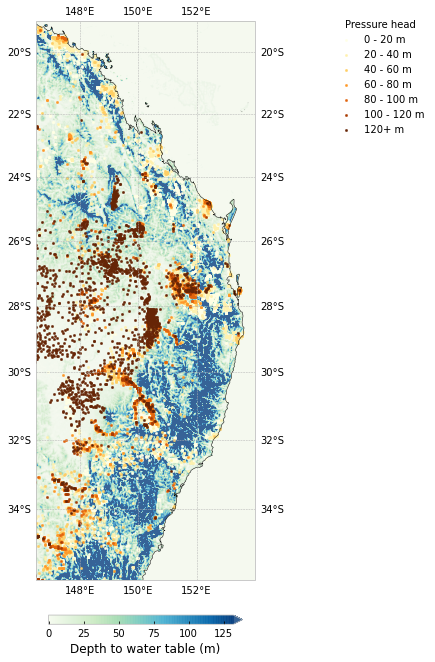
Data Assimilation
2) Hydraulic Pressure Head
Groundwater
observation well
Cl recharge observation
layer 1
layer 2
layer 3
Misfit
Data Assimilation
2) Hydraulic Pressure Head
3) Temperature gradients
1) Chloride concentration
Data Assimilation
3) Temperature gradients
Temperature borehole
Misfit
layer 1
layer 2
layer 3
Coal seam
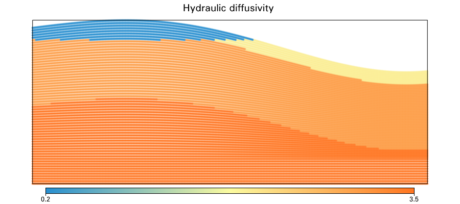
Thermal conductivity
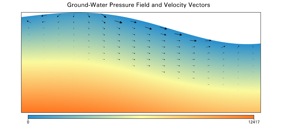
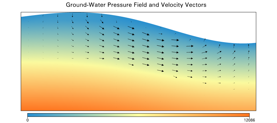
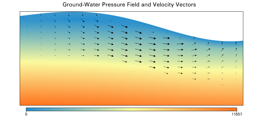
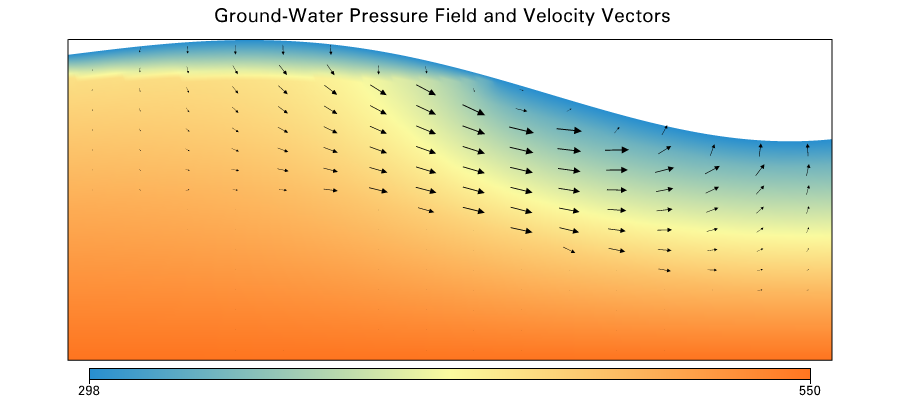
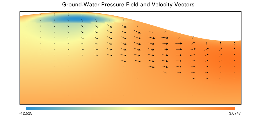
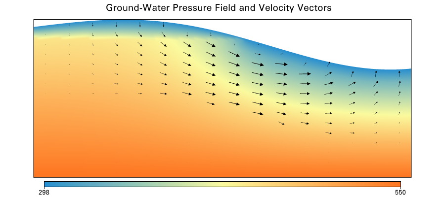
Temperature field with groundwater velocity vectors
Fluid flow off
Fluid flow on
Difference
Data Assimilation
3) Temperature gradients
2) Hydraulic Pressure Head
1) Chloride concentration
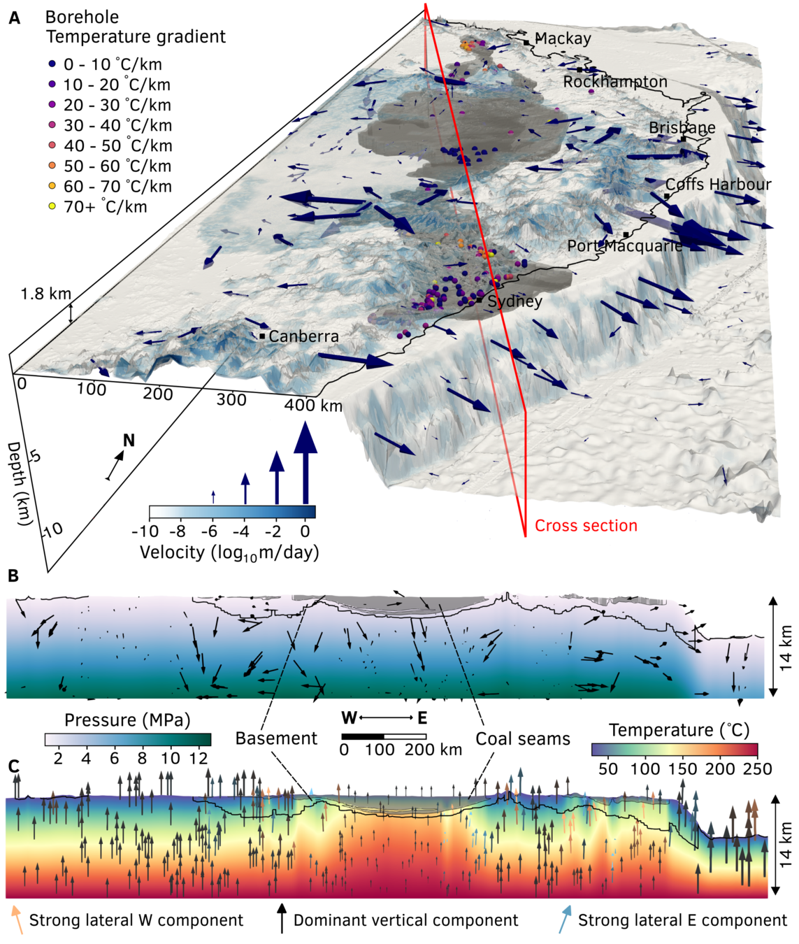
High discharge rates off the continental shelf
- up to 3 m/day
Very long residence times inland (383 ka) compared to coastal aquifers (182 a)
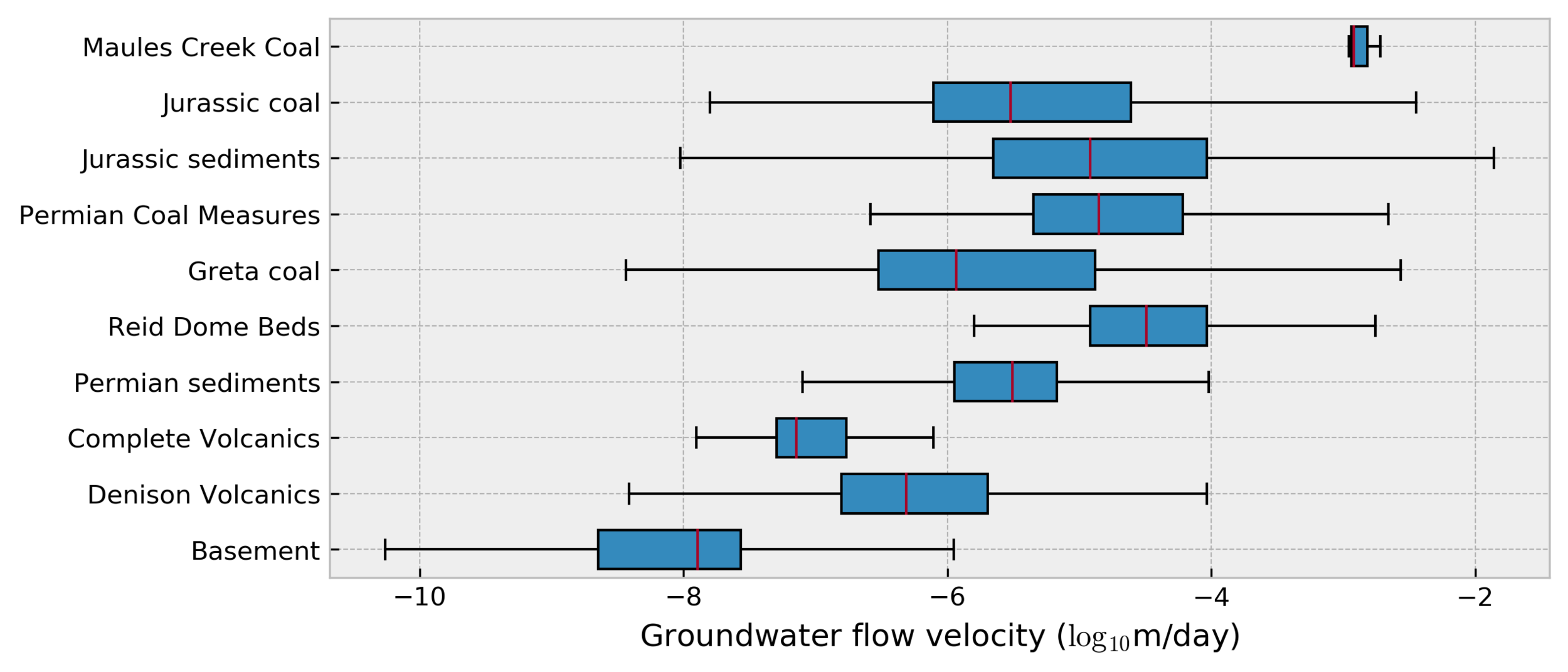
Groundwater flow velocities for each
geological layer in our 3D model
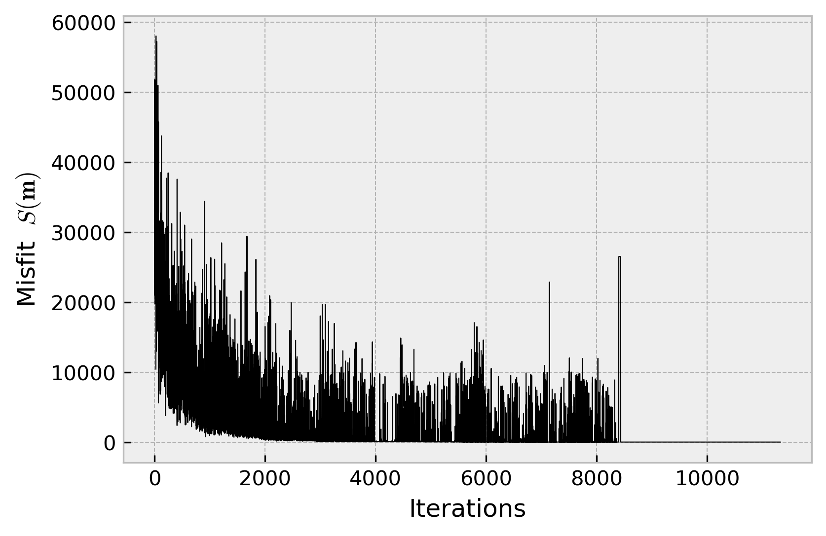
Misfit with respect to model iterations.
We reach convergence at approximately 8500 iterations.
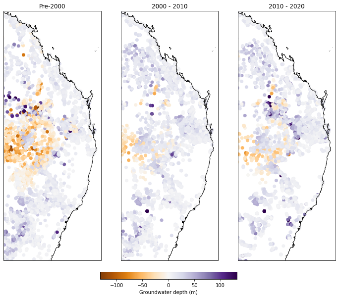
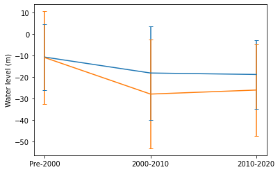
Water level 2000-2020
Thank you
Dr. Ben Mather
Madsen Building, School of Geosciences,
The University of Sydney, NSW 2006