Reducing the uncertainty of lithospheric thermal structure
integrated modelling from geothermal, magnetic, and seismic data



Dr. Ben Mather
EarthByte Group & Sydney Informatics Hub
Motivation
Understanding temperature in the crust can help to interpret:
- hydrocarbon maturity
- geothermal potential
- seismic velocity
Quantifying its uncertainty is important to estimate the risk associated with a resource
Bayesian Inference
Posterior ~ likelihood x prior
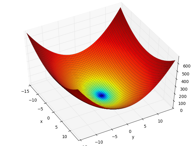
-norm objective function
- Bayes theorem describes the posterior as the probability of a model given the data
- The posterior probability can be evaluated with an objective function
- We seek the maximum a posteriori (MAP) model, which can be obtained by minimising S(m).
Adjoint inversion
Efficiently invert a large number of parameters
Added complexity to compute forward problem AND gradient vectors
Entrapment by local minima
Number of evaluations increase exponentially with dimensions
Copes better with highly nonlinear problems
Posterior distribution
MCMC
Adjoint
+
+
+
-
-
-
Thermal solver
Objective function
Input parameters


Forward
Model
Adjoint
Model
Gradient descent
The gradient descent method for finding successibely better approximations to the minimum of S(m) is:
However, we use a quasi-Newton nonlinear solver to approximate the Hessian (2nd derivatives)
- Useful because the Hessian is difficult to compute
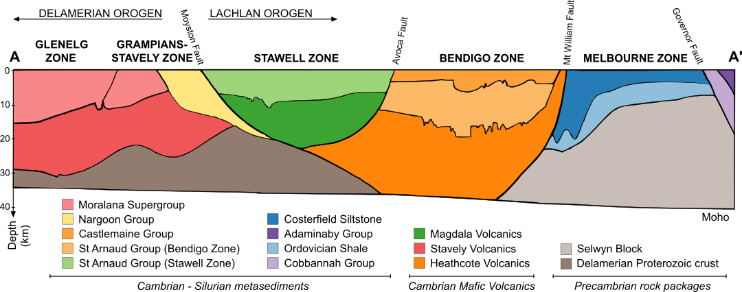
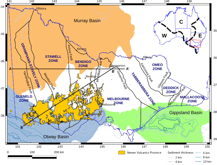
Regional context
SE Australia is an accretionary terrane combining Proterozoic and Phanerozoic crust
A
A'
Data assimilation
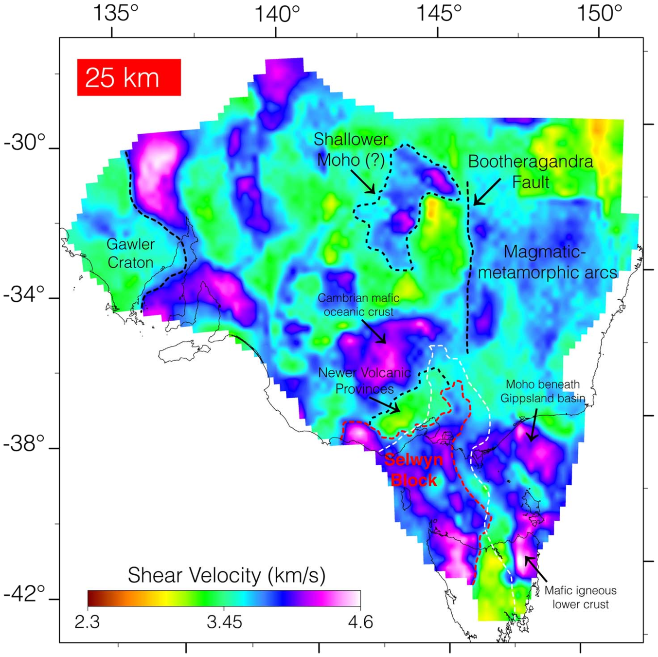
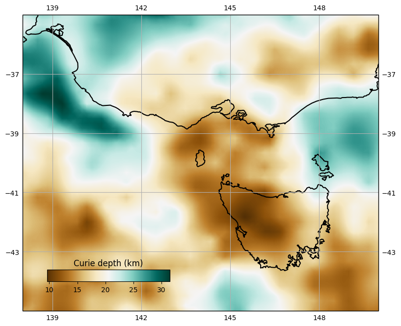
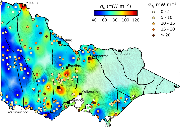
- On their own, any of these datasets result in non-unique solutions of temperature.
- Together, they constrain temperature in the lithosphere to a reasonable degree of uncertainty.
HEAT FLOW
CURIE DEPTH
SHEAR VELOCITY

Uncertainty reduction
Coupling gradient inversion with local sampling builds an approximation of the posterior
- Perturb observation within PDF
- Perturb priors within PDF
- Build the ensemble
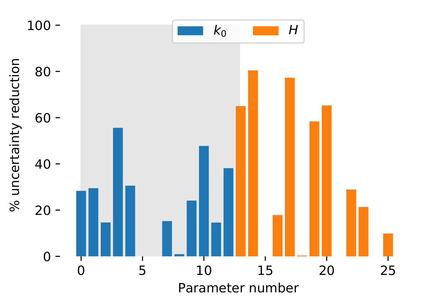
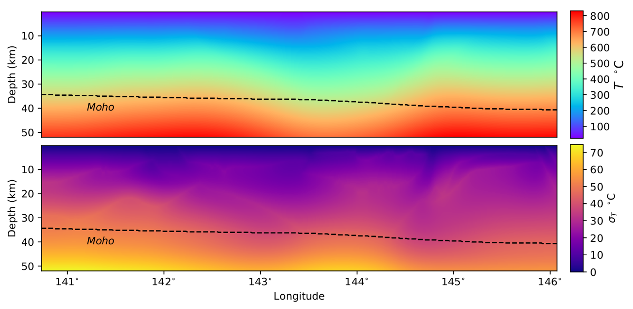
Uncertainty reduction
MAP estimate
Standard deviation
thermal
conductivity
heat production
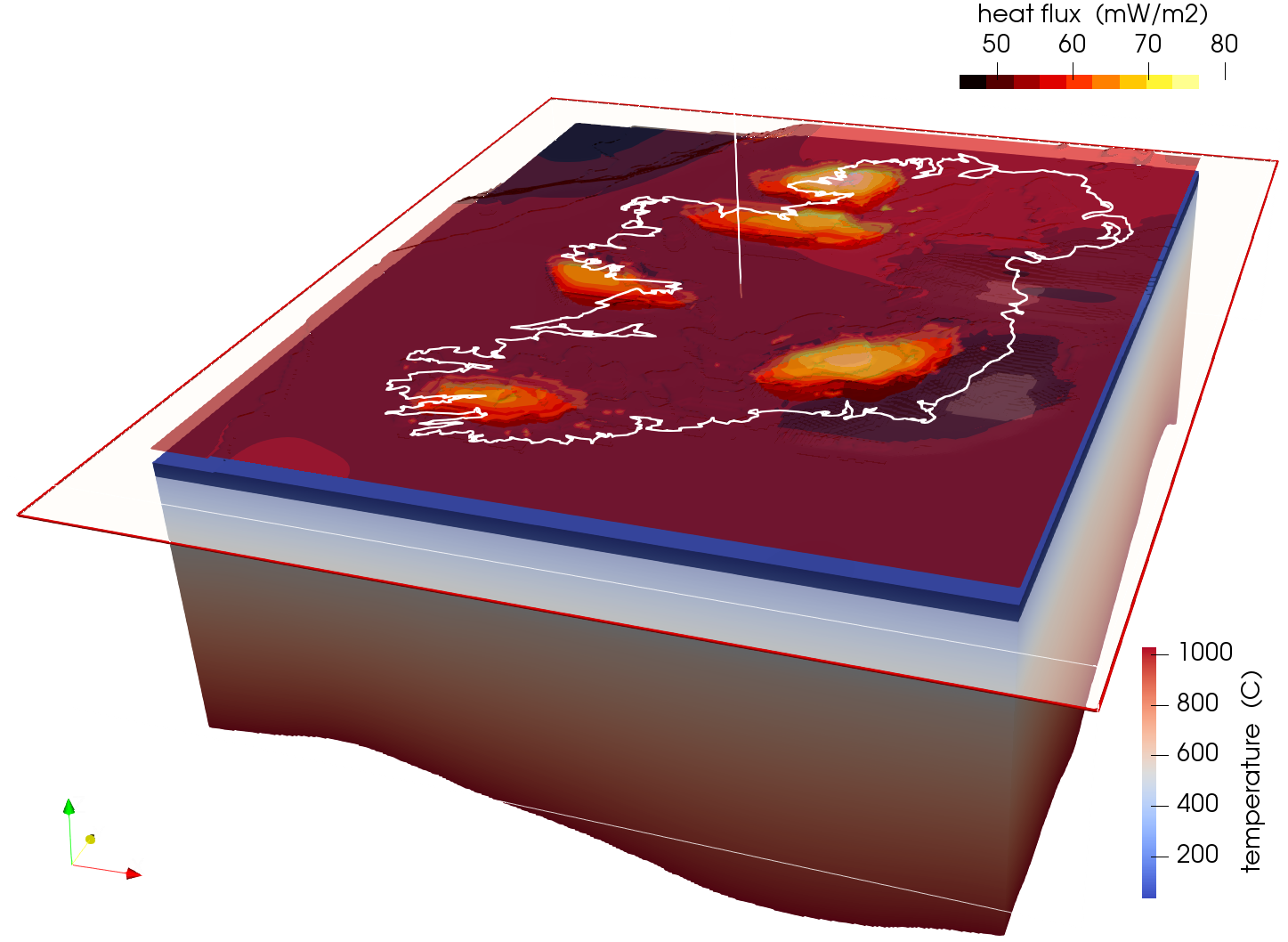
Thermal model of Ireland
- Significant heat refraction in Northern Ireland.
- High temperature related to lateral branch of Iceland plume(?)
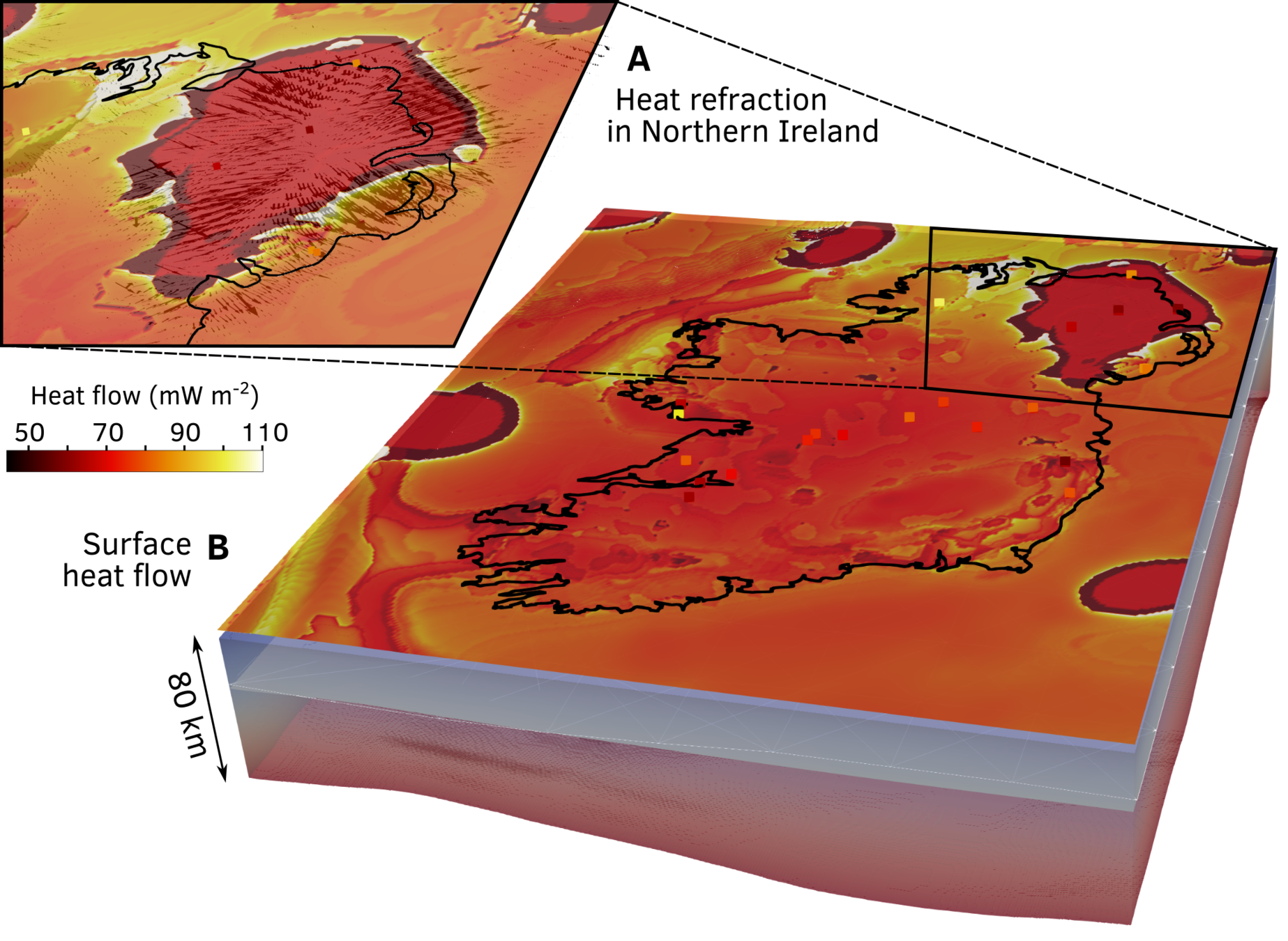
Temperature model with surface heat flow
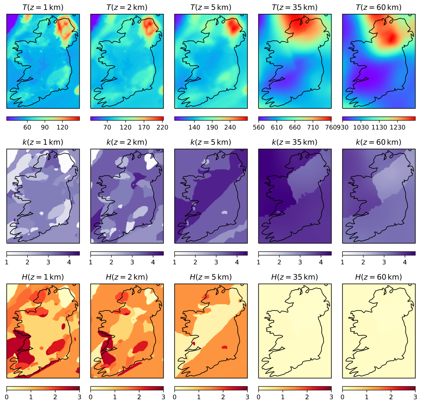
Temperature, thermal conductivity, heat production
at various depths
Thank you
Dr. Ben Mather
Madsen Building, School of Geosciences,
The University of Sydney, NSW 2006