pyBadlands workshop
Docker image
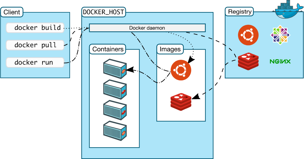
Docker image
$ docker pull brmather/pybadlands-workshop:18.04-ubuntu
$ docker images
REPOSITORY                            TAG                 IMAGE ID            CREATED             SIZE
brmather/pybadlands-workshop          18.04-ubuntu        0f196ceade6d        5 hours ago         3.17GB
brmather/pybadlands-workshop-base     18.04-ubuntu        17a94e4b836a        2 days ago          1.7GB
$
$ docker run --name pybadlands -p 8888:8888 brmather/pybadlands-workshop:18.04-ubuntu
$ docker ps
CONTAINER ID        IMAGE                                       COMMAND                  CREATED             STATUS              PORTS                              NAMES
d553869450dc        brmather/pybadlands-workshop:16.04-ubuntu   "/usr/local/bin/tini…"   5 hours ago         Up 5 hours          9999/tcp, 0.0.0.0:8885->8888/tcp   pybadlands-workshop
Pull the docker image to your computer and run it within a container
Binder
Alternatively, load the workshop in the cloud with Binder
IMPORTANT: Binder does not save your work and will time-out after a period of inactivity.
If everything went well, you should see this...
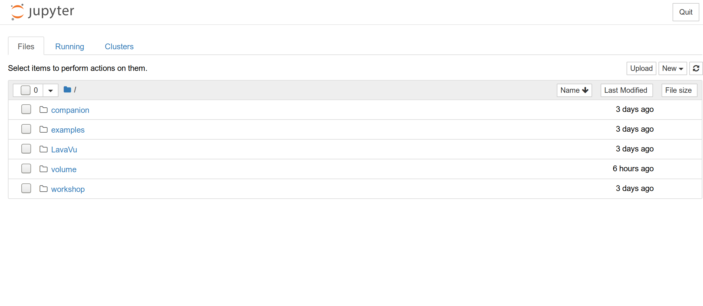
navigate to examples
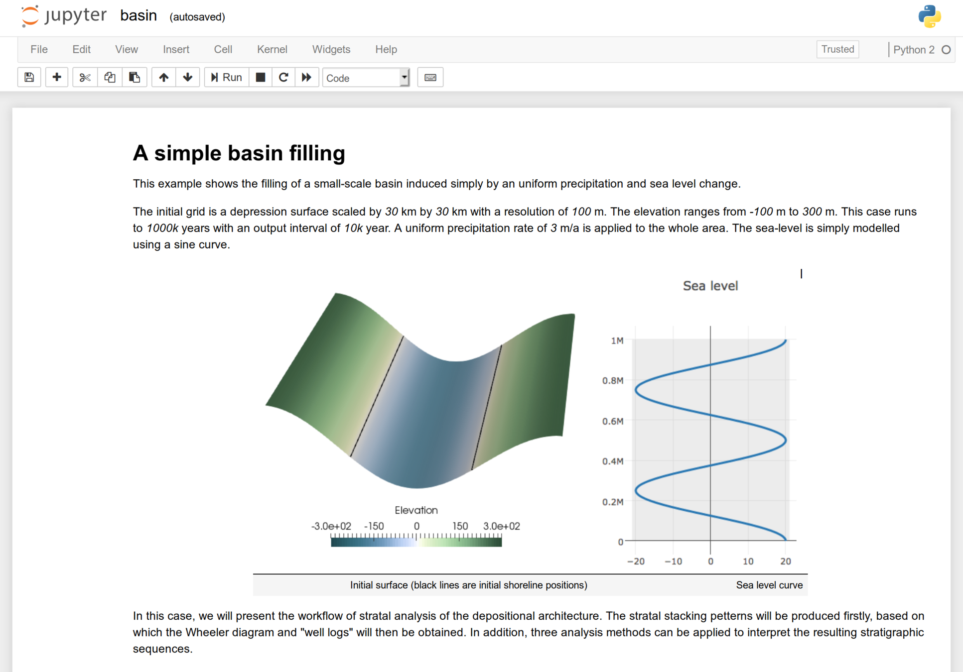
Example 1: basin
- Generate topographic grid
- Build sea level curve
- Run time series
badlands model - basin.xml
<?xml version="1.0" encoding="UTF-8"?>
<badlands xmlns:xsi="http://www.w3.org/2001/XMLSchema-instance">

    <!-- Regular grid structure -->
    <grid>
        <!-- Digital elevation model file path -->
        <demfile>data/node.csv</demfile>
        <!-- Boundary type: flat, slope, fixed or wall -->
        <boundary>fixed</boundary>
        <!-- Optional parameter (integer) used to decrease TIN resolution.
             The default value is set to 1. Increasing the factor
             value will multiply the digital elevation model resolution
             accordingly.  -->
        <resfactor>1</resfactor>
    </grid>

    <!-- Simulation time structure -->
    <time>
        <!-- Simulation start time [a] -->
        <start>0.</start>
        <!-- Simulation end time [a] -->
        <end>1000000.</end>
        <!-- Display interval [a] -->
        <display>10000.</display>
    </time>

    <!-- Simulation stratigraphic structure -->
    <strata>
        <!-- Stratal grid resolution [m] -->
        <stratdx>100.</stratdx>
        <!-- Stratal layer interval [a] -->
        <laytime>10000.</laytime>
    </strata>

    <!-- Sea-level structure -->
    <sea>
        <!-- Relative sea-level position [m] -->
        <position>0.</position>
        <!-- Sea-level curve - (optional) -->
        <curve>data/sealevel.csv</curve>
        <!-- Limit flow network computation based on
             water depth [m] -->
        <limit>200.</limit>
    </sea>

    <!-- Precipitation structure -->
    <precipitation>
        <!-- Number of precipitation events -->
        <climates>1</climates>
        <!-- Precipitation definition -->
        <rain>
            <!-- Rain start time [a] -->
            <rstart>0.</rstart>
            <!-- Rain end time [a] -->
            <rend>1000000.</rend>
            <!-- Precipitation value [m/a] - (optional) -->
            <rval>3.</rval>
        </rain>
    </precipitation>

    <!-- Stream power law parameters:
         The stream power law is a simplified form of the usual expression of
         sediment transport by water flow, in which the transport rate is assumed
         to be equal to the local carrying capacity, which is itself a function of
         boundary shear stress. -->
    <sp_law>
        <!-- Make the distinction between purely erosive models (0) and erosion /
            deposition ones (1). Default value is 1 -->
        <dep>1</dep>
        <!-- Critical slope used to force aerial deposition for alluvial plain,
             in [m/m] (optional). -->
        <slp_cr>0.001</slp_cr>
        <!-- Maximum percentage of deposition at any given time interval from rivers
             sedimentary load in alluvial plain. Value ranges between [0,1] (optional). -->
        <perc_dep>0.75</perc_dep>
        <!-- Planchon & Darboux filling thickness limit [m]. This parameter is used
              to defined maximum accumulation thickness in depression area per time
              step. Default value is set to 1. -->
        <fillmax>50.</fillmax>
        <!-- Values of m and n indicate how the incision rate scales
             with bed shear stress for constant value of sediment flux
             and sediment transport capacity.
             Generally, m and n are both positive, and their ratio
             (m/n) is considered to be close to 0.5 -->
        <m>0.5</m>
        <n>1.0</n>
         <!-- The erodibility coefficient is scale-dependent and its value depend
             on lithology and mean precipitation rate, channel width, flood
             frequency, channel hydraulics. In case where the erodibility
             structure is turned on, this coefficient is applied to the reworked
             sediments. -->
        <erodibility>9.e-7</erodibility>
        <!-- Number of steps used to distribute marine deposit.
             Default value is 5 (integer). (optional)-->
        <diffnb>5</diffnb>
        <!-- Proportion of marine sediment deposited on downstream nodes. It needs
             to be set between ]0,1[. Default value is 0.9 (optional). -->
        <diffprop>0.2</diffprop>
    </sp_law>

    <!-- Linear slope diffusion parameters:
         Parameterisation of the sediment transport includes the simple creep transport
         law which states that transport rate depends linearly on topographic gradient. -->
    <creep>
        <!-- Surface diffusion coefficient [m2/a] -->
        <caerial>2.5e-2</caerial>
        <!-- Marine diffusion coefficient [m2/a] -->
        <cmarine>5.e-2</cmarine>
        <!-- River transported sediment diffusion
             coefficient in marine realm [m2/a] -->
        <criver>5.</criver>
    </creep>

    <!-- Output folder path -->
    <outfolder>output</outfolder>

</badlands>
Visualisation in Paraview
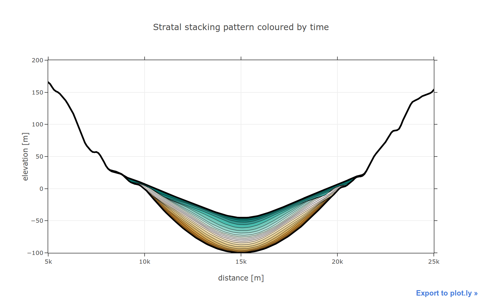
strataAnalyse_basin.ipynb
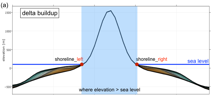
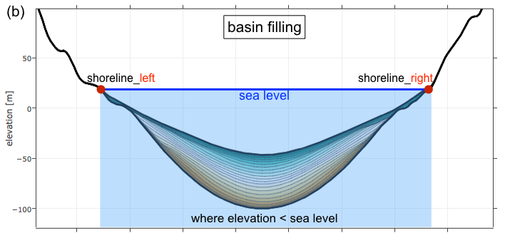
Analyse stratigraphic output
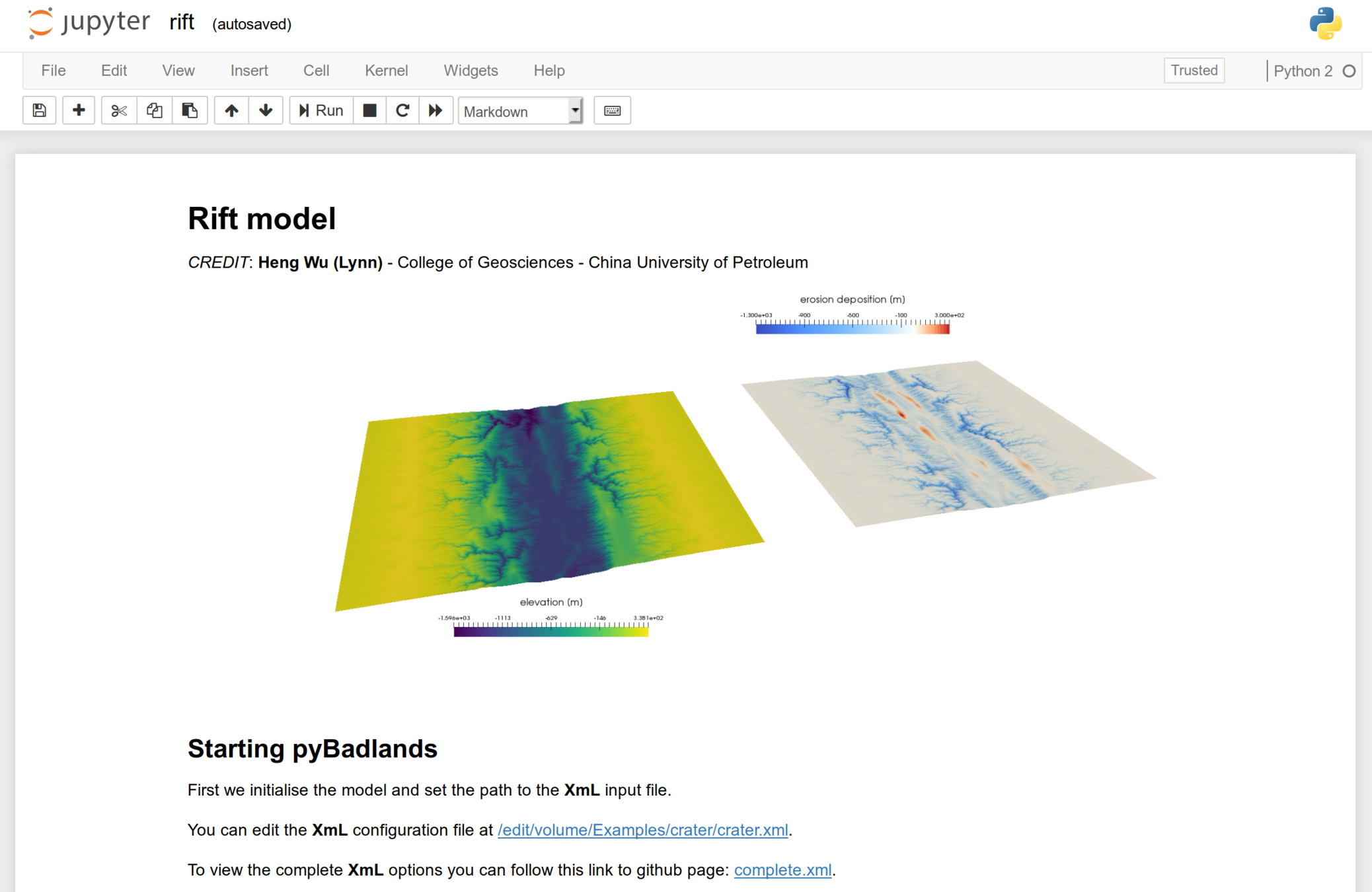
Example 2: rift
Explore the erosion and deposition effects associated with rifting.