Learn Dynamics with Diffusion Forcing
Boyuan Chen
Path to General EI: world models
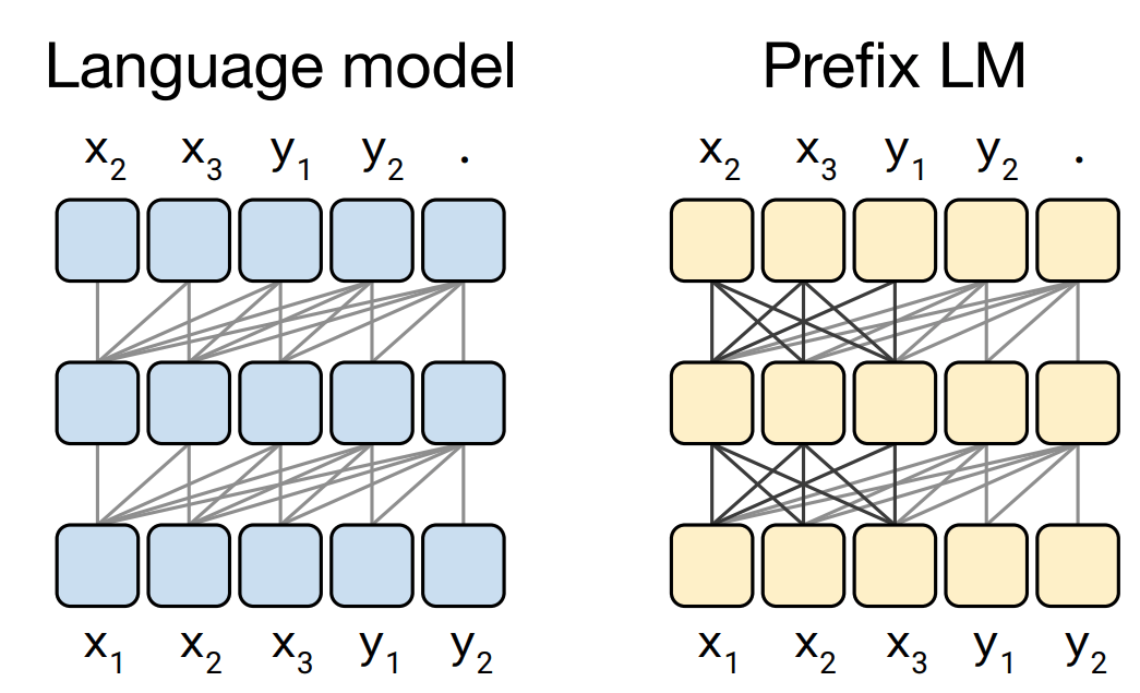
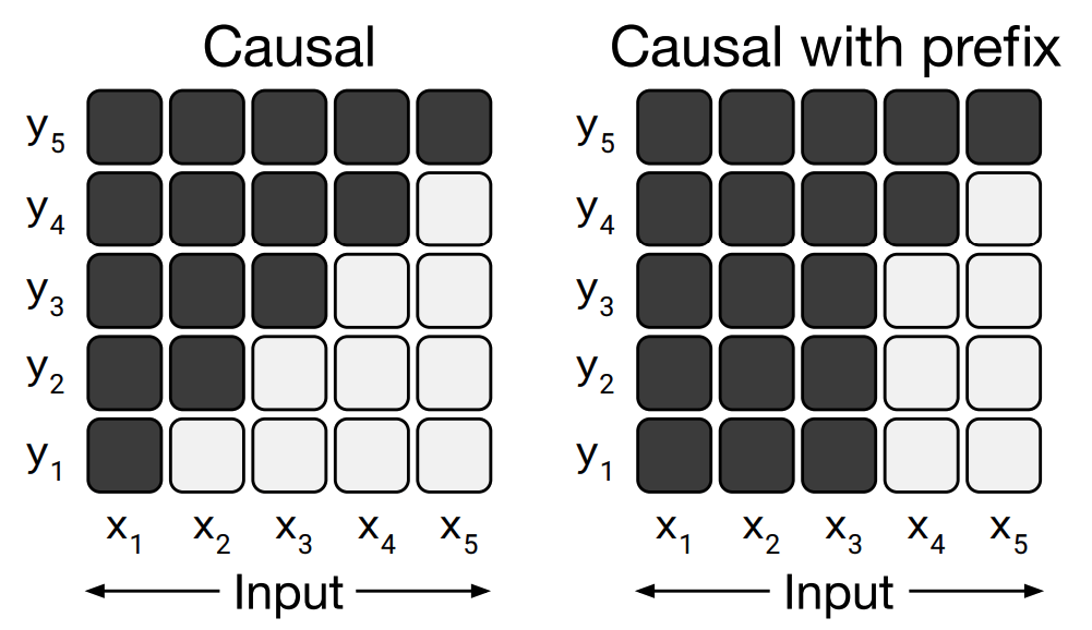
Auto Regressive Models
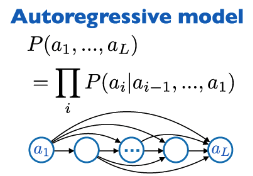
Auto Regressive Models
- Flexible horizon
- Causal correctness
- better capture likelihood of "single-step transition"
- Better compositionality
- More efficient for search
Whole Sequence Diffusion

Whole Sequence Diffusion
- Flexible conditioning at test time wo/ retraining
- Guidance over long horizon (for planning)
- Better capture global, joint distribution
Auto Regressive Models
- Flexibility
- Capture causal dynamics
Whole Sequence Diffusion
- Long horizon guidance
- Capture global likelihood
Get good from both!
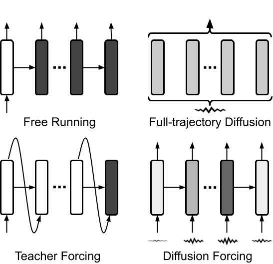
Diffusion Forcing (final name TBD) is a probabilistic sequence model that interleaves time axis of auto-regressive models and noise-level axis of diffusion models.
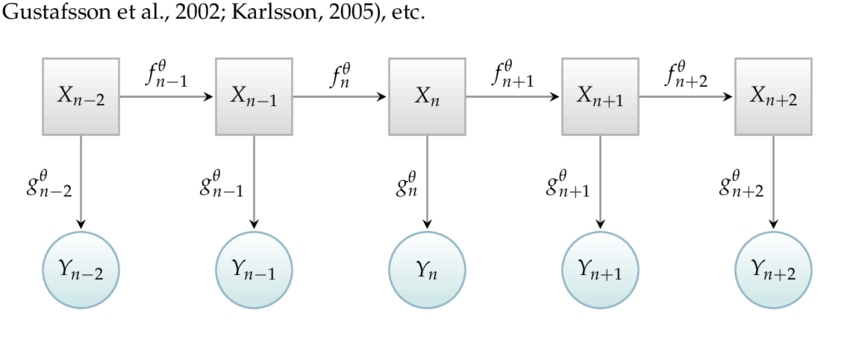
Prelim: Bayes Filter
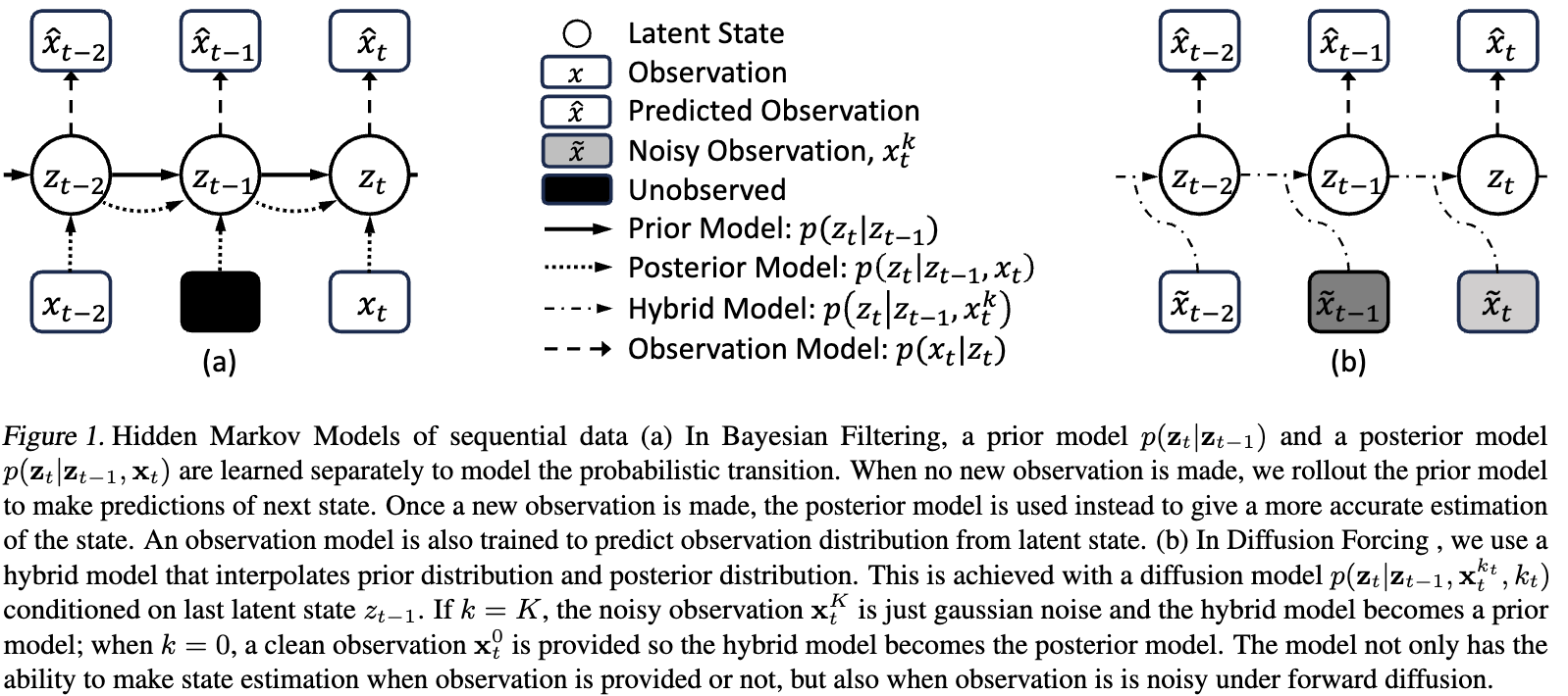
Prior Model to predict state when there is no updated observation
Prelim: Bayes Filter
Posterior Model to predict state when new observation is made
What if we relax bayes filter from the binary duo of having an observation vs no observation?
No observation -> Noisy observation -> Has observation
Core idea: masking by noise
Masking is a fundamental technique in self-supervised learning
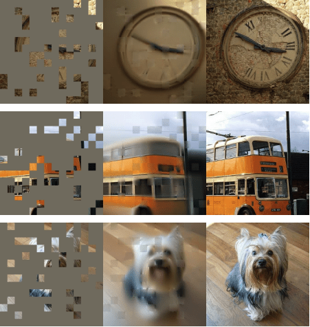
Core idea: masking by noise
What if we mask by noise, instead of zero padding?
Masked
Not masked
partially masked
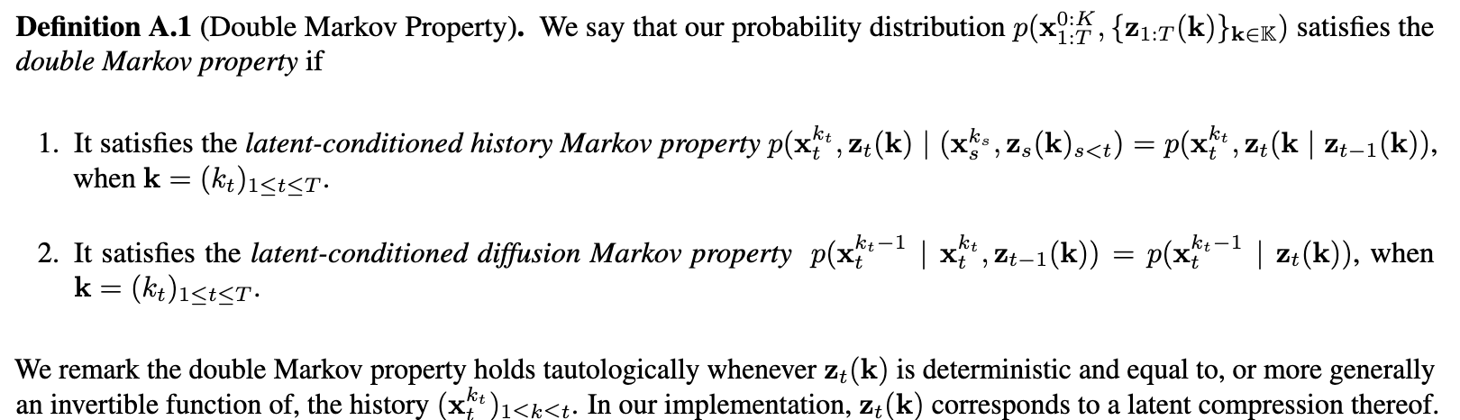
Diffusion Forcing
Diffusion
Step (k)
Time step (t)
Diffusion Forcing
Noise
level (k)
Time step (t)
Diffusion Forcing
Diffusion Forcing
Diffusion Forcing
Diffusion Forcing
What does this give us:
We can diffuse a frame at far future, without fully diffusing the past!
(because we are trained on it)
Diffusion Forcing
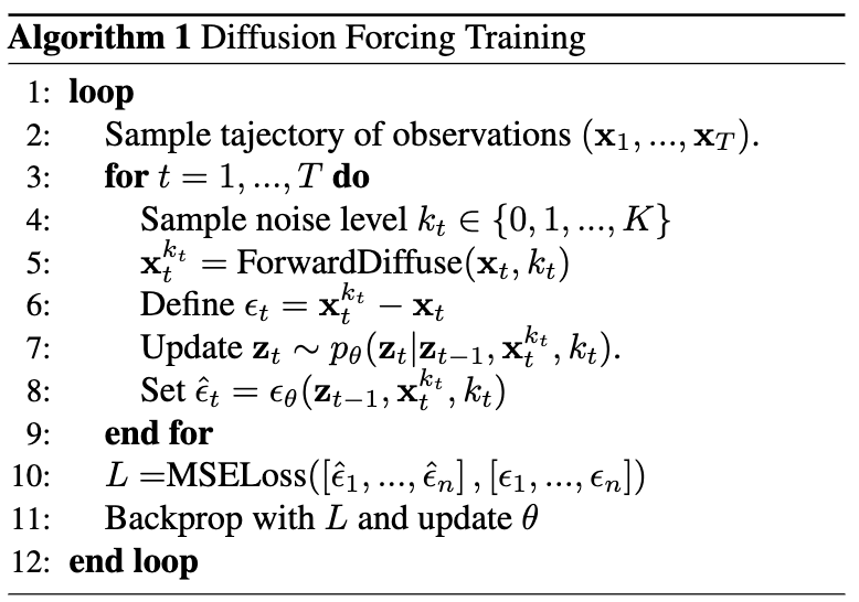
And after two pages of math

Comparison
RNN is all you need?
50%
50%
RNN is all you need?
Optimal one step prediction in state space
with deterministic model
RNN is all you need?
Optimal one step prediction in pixel space
with deterministic model
RNN is all you need?


Imitate human trajectories
RNN is all you need?
Imitate human trajectories with deterministic model
Solution: Learn Distribution
Variational Inference
Variational Inference
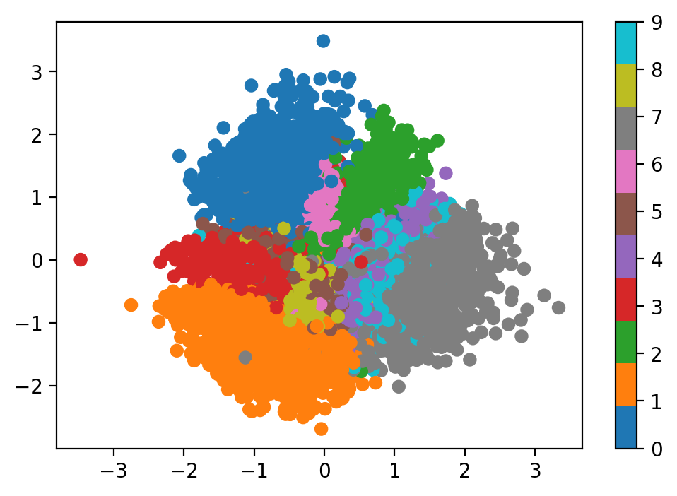
A distribution we know
how to sample from
A distribution we know
how to sample from
target distribution
Types of variational model
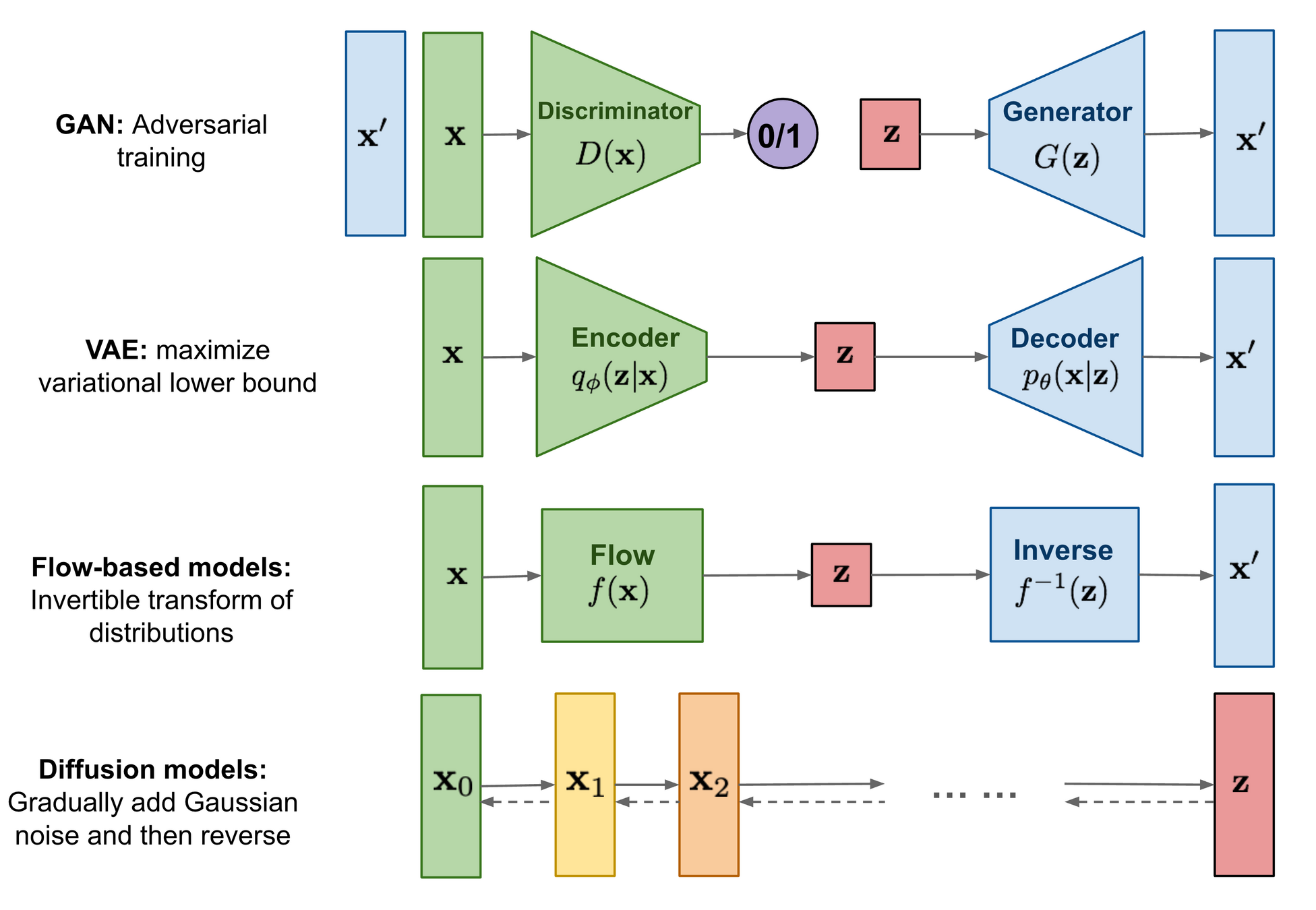
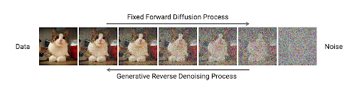
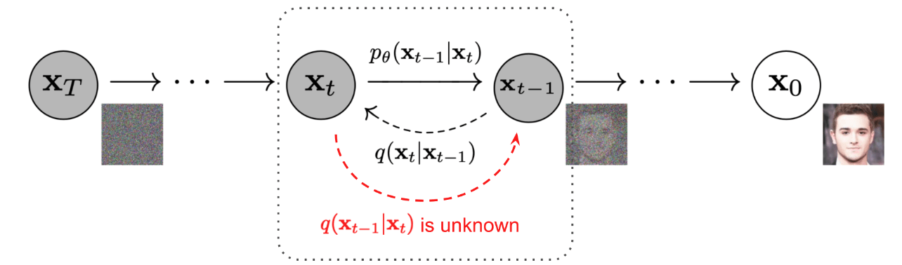
Diffusion Model

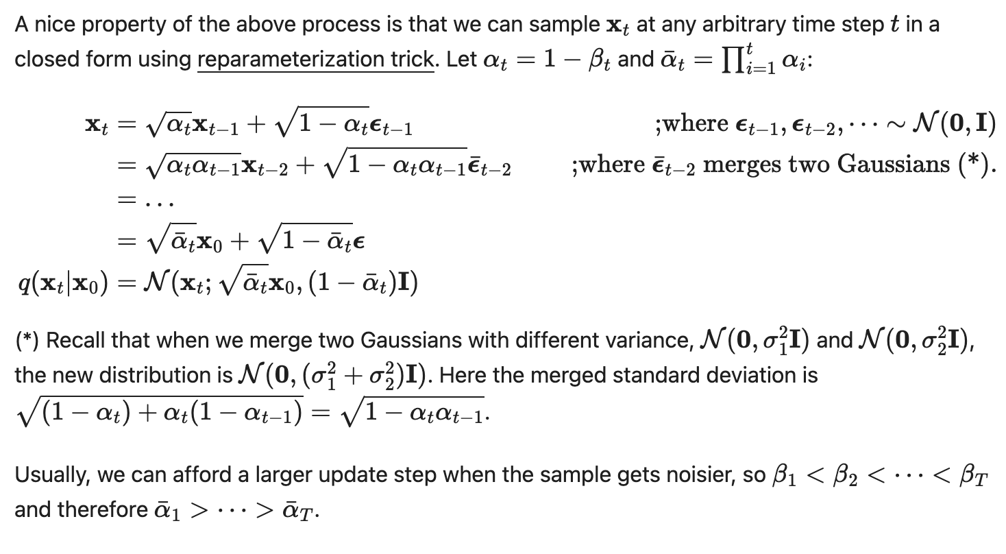
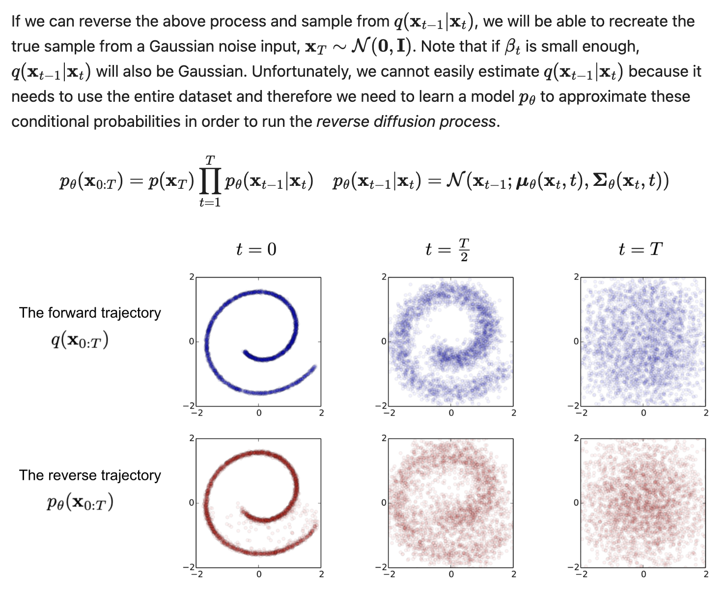
Forward Diffusion process
Forward Diffusion process
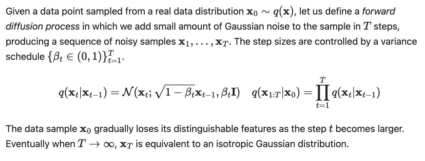
Forward Diffusion process
Reverse Diffusion process
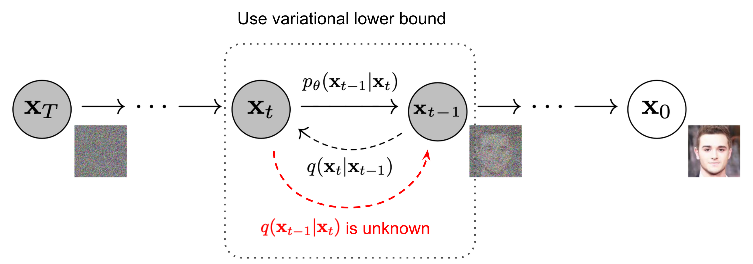
Reverse Diffusion process
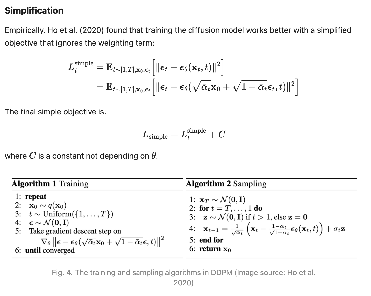
Diffusion Training

Diffusion Training
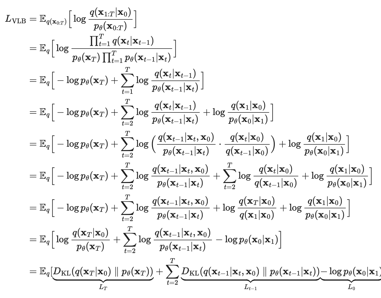
Diffusion Training
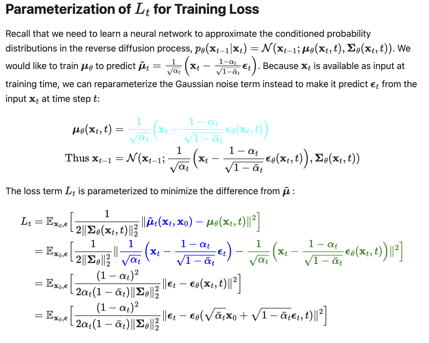
Diffusion Training
Conditional Diffusion
Let y be a variable we want to condition on, e.g. y=a label='cat'
Conditional Diffusion
Let y be a variable that's learned? Yes!
It could be a differentiable latent code that encodes belief given all previous observations.

Warning!
Change of notation
Steps in diffusion are usually denoted by t. But from now on we will denote it as k, as we will introduce the actual time variable, t.
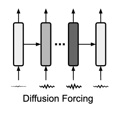
How to learn stochastic dynamics?
How to learn stochastic dynamics?
Learn dynamics and control with
Diffusion Forcing
Diffusion Forcing is a sequence model that
- have out-standing performance on continuous sequence modeling
- is a state-space model that's strictly markovian
- has explicit control over context length and thus compositionality
- has explicit control over generation horizon
- can take advantage of noisy observations
has explicit control over generation horizon

Full Trajectory rollout
Single step rollout
Our method can do both
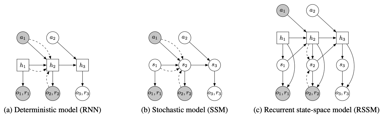
State Space Models
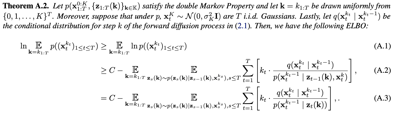
ELBO 1
Given initial context \(s_0\) (ommited in notation for simplicity)
$$ \ln p(o_{1:T})=\ln\int_{s_{1:T}}p(o_{1:T},s_{1:T}) \ d{s_{1:T}}$$
$$=\ln\int_{s_{1:T}} \prod_{t=1}^T p(o_t,s_t|s_{1:t-1},o_{1:t-1}) \ d{s_{1:T}}$$
$$=\ln\int_{s_{1:T}} \prod_{t=1}^T p(o_t|s_{1:t},o_{1:t-1}) p(s_t|s_{1:t-1},o_{1:t-1}) \ d{s_{1:T}}$$
$$=\ln\int_{s_{1:T}} \prod_{t=1}^T p(o_t|s_{t}) p(s_t|s_{t-1}) \ d{s_{1:T}}$$
$$=\ln\mathop{\mathbb{E}}_{s_{1:T}}[\prod_{t=1}^T p(o_t|s_{t})] $$
ELBO 1
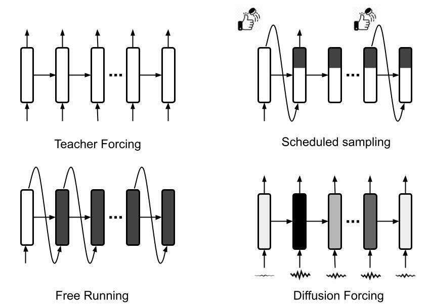
How to sample \( s_{1:T}\) as in the expectation \(\mathop{\mathbb{E}}_{s_{1:T}}[\prod_{t=1}^T p(o_t|s_{t})]\)? Candidate: free-running rollout
\(p(o_{1:T})=\ln\mathop{\mathbb{E}}_{s_{1:T}}[\prod_{t=1}^T p(o_t|s_{t})]\ge \sum_{t=1}^T \mathop{\mathbb{E}}_{s_{1:T}}[\ln p(o_t|s_{t})]\)
ELBO 2
What about importance sampling with posterior
$$\ln p(o_{1:T}) = \ln \mathop{\mathbb{E}}_{s_{1:T}}[\prod_{t=1}^T p(o_t|s_{t})]=\ln \mathop{\mathbb{E}}_{s_t\sim p(s_t|s_{t-1})}[\prod_{t=1}^T p(o_t|s_{t})]$$
$$=\ln\mathop{\mathbb{E}}_{s_t\sim p(s_t|s_{t-1},o_t)}[\prod_{t=1}^T p(o_t|s_{t}) p(s_t|s_{t-1}) / p(s_t|s_{t-1},o_t)]$$
$$=\ln\mathop{\mathbb{E}}_{s_t\sim p(s_t|s_{t-1},o_t)}[\prod_{t=1}^T p(o_t,s_t|s_{t-1}) / p(s_t|o_t,s_{t-1})]$$
$$=\ln\mathop{\mathbb{E}}_{s_t\sim p(s_t|s_{t-1},o_t)}[\prod_{t=1}^T p(o_t|s_{t-1}) ]$$
ELBO 2
$$\ln p(o_{1:T}) =\ln\mathop{\mathbb{E}}_{s_t\sim p(s_t|s_{t-1},o_t)}[\prod_{t=1}^T p(o_t|s_{t-1}) ]$$
$$\ge \mathop{\mathbb{E}}_{s_t\sim p(s_t|s_{t-1},o_t)}[\ln(\prod_{t=1}^T p(o_t|s_{t-1}) ])$$
$$\ge \mathop{\mathbb{E}}_{s_t\sim p(s_t|s_{t-1},o_t)}[\sum_{t=1}^T \ln p(o_t|s_{t-1}) ])$$
Where each \(p(o_t|s_{t-1})\) can be lower bounded
by ELBO of diffusion models, conditioned on s_{t-1}!
ELBO 2
\(\ln p(o_{1:T})\ge \mathop{\mathbb{E}}_{s_t\sim p(s_t|s_{t-1},o_t)}[\sum_{t=1}^T \ln p(o_t|s_{t-1}) ])\)
We can do importance sampling via teacher forcing
Compare ELBO 1 & 2
ELBO1: \(\ln p(o_{1:T})\ge \sum_{t=1}^T \mathop{\mathbb{E}}_{s_t\sim p(s_t|s_{t-1})}[\ln p(o_t|s_{t})]\)
ELBO2: \(\ln p(o_{1:T})\ge \sum_{t=1}^T \mathop{\mathbb{E}}_{s_t\sim p(s_t|s_{t-1},o_t)}[ \ln p(o_t|s_{t-1}) ])\)
ELBO1 samples from prior model \(p(s_t|s_{t-1})\)
ELBO2 samples from posterior model \( p(s_t|s_{t-1},o_t)\)
What about something in between? \( p(s_t|s_{t-1},N(o_t))\), where N(o_t) is a noised version of \(o_t\)
Diffusion Forcing
What about something in between?
\( p(s_t|s_{t-1},N(o_t))\), where \(N(o_t)\) is a noised version of \(o_t\)
\( p(s_t|s_{t-1},N(o_t)) \rightarrow p(s_t|s_{t-1},o_t)\) when \(N\) is zero noise
\( p(s_t|s_{t-1},N(o_t)) \rightarrow p(s_t|s_{t-1},o_t)\) when \(N(o_t)\) is pure noise
We constructed a smooth interpolation between prior and posterior!
Diffusion Forcing (ours)
Diffusion Forcing Sampling
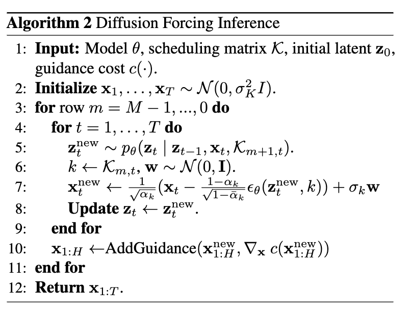
Diffusion Forcing Sampling (horizon 1)
Diffusion
Step (k)
Time step (t)
Diffusion Forcing Sampling (horizon ∞)
Diffusion
Step (k)
Time step (t)
Diffusion Forcing Sampling (pyramid)
Diffusion
Step (k)
Time step (t)
Account for uncertainty under causal dynamics
Diffusion
Step (k)
Time step (t)
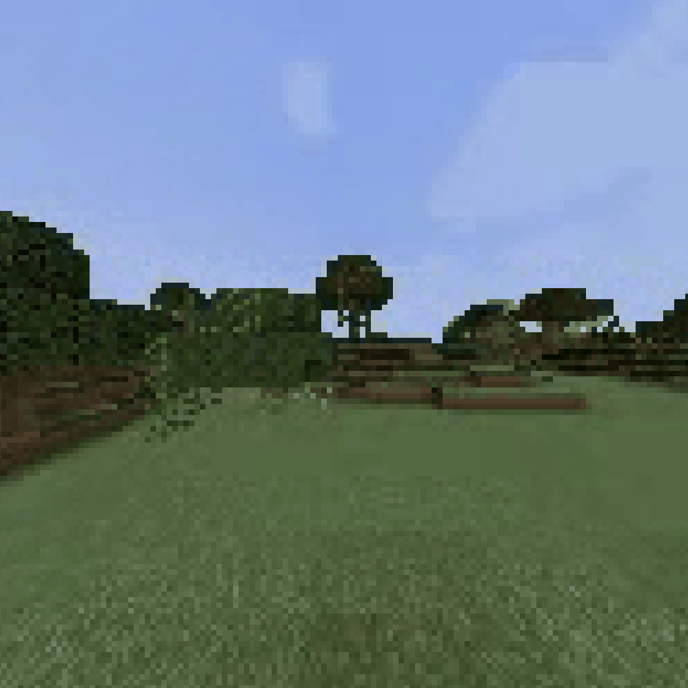
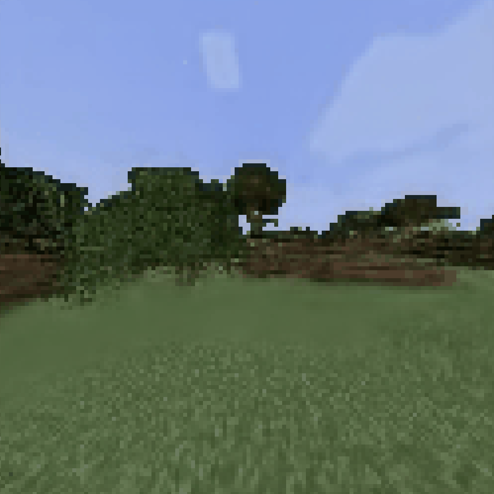
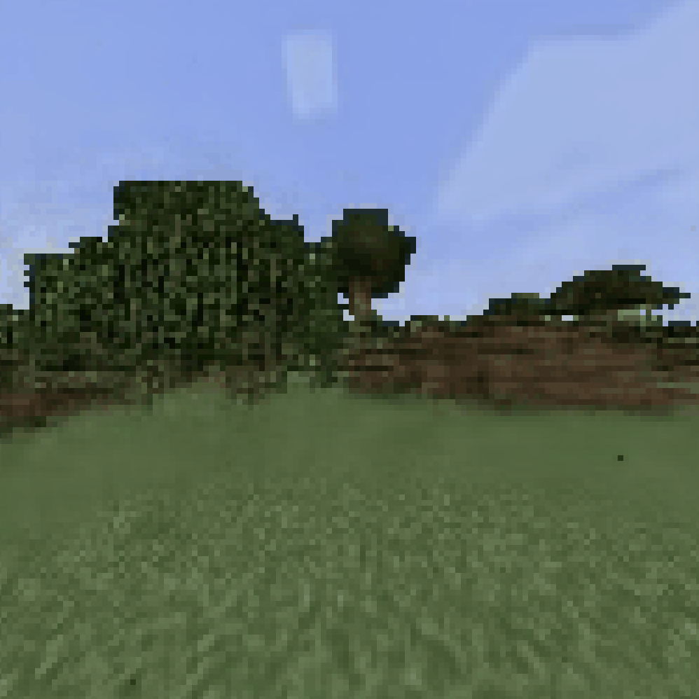
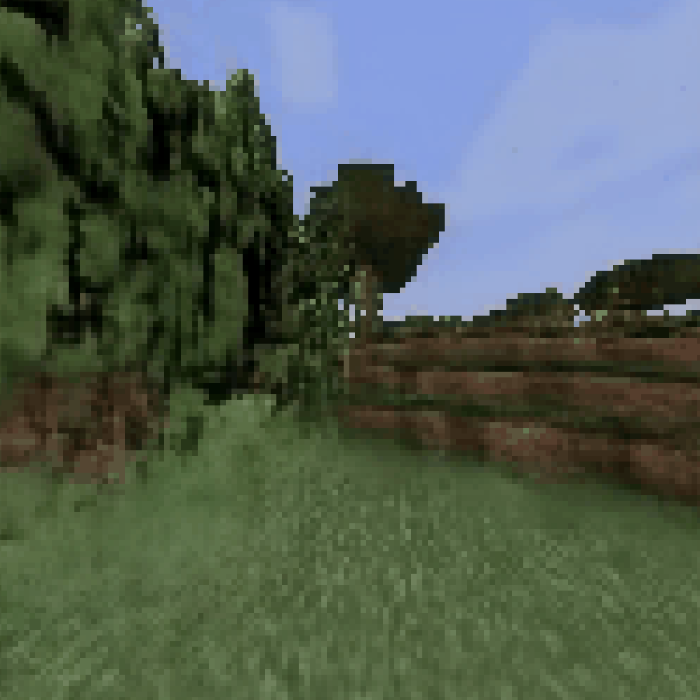
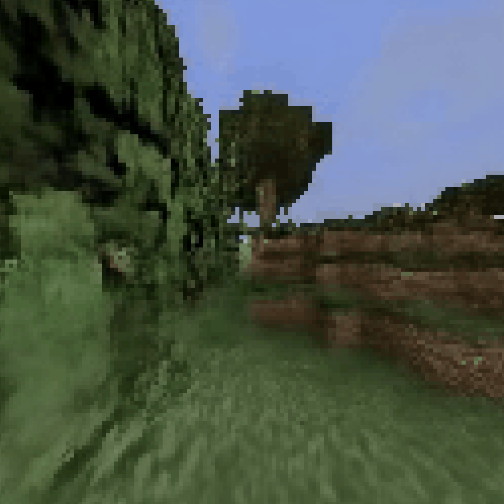
Video Prediction (72 frames)
Generated vs GT
Video Prediction (72 frames)


Generated vs GT
Infinite Rollout
train on 72, sample on 500 without sliding window
(500 is due to gif size, can do 3000+ wo blowing up)
64x64

128x128
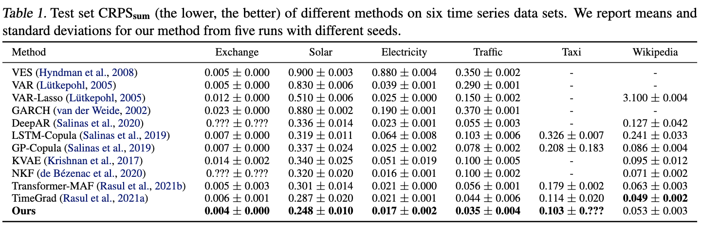
Time Series Prediction
Control over context-horizon and compositionality
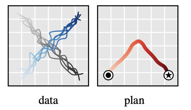
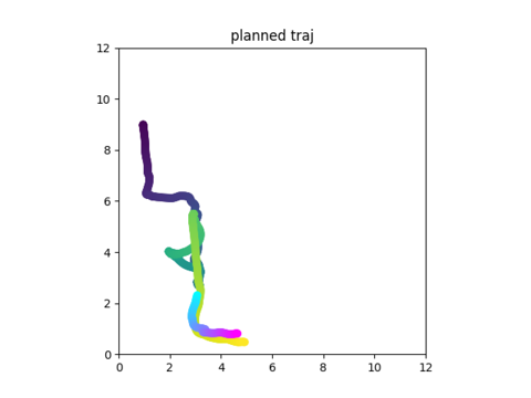
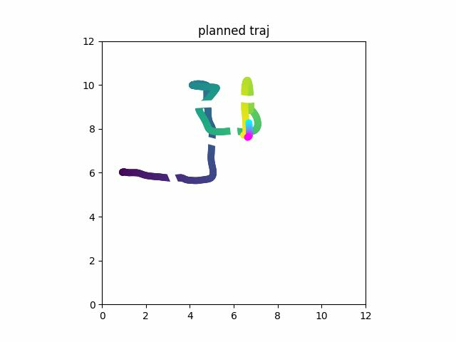
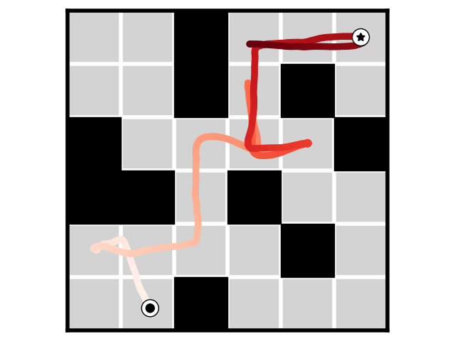
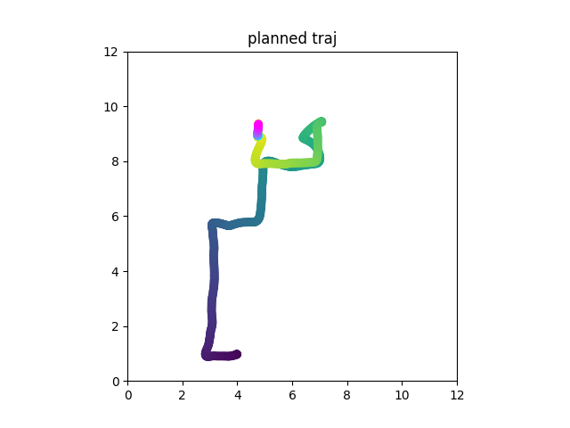
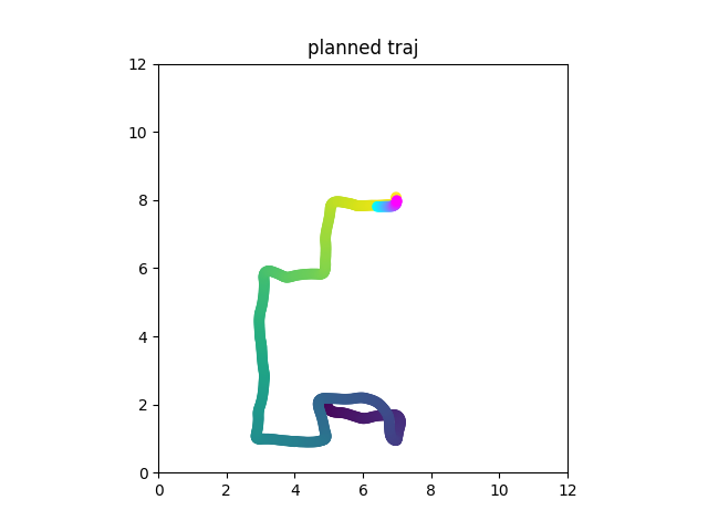
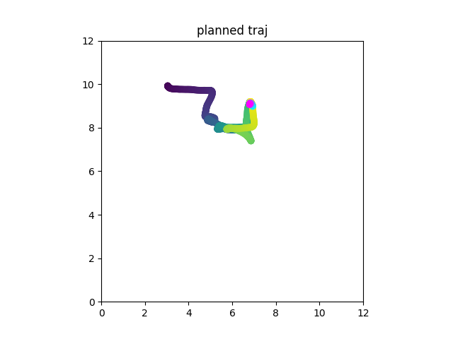
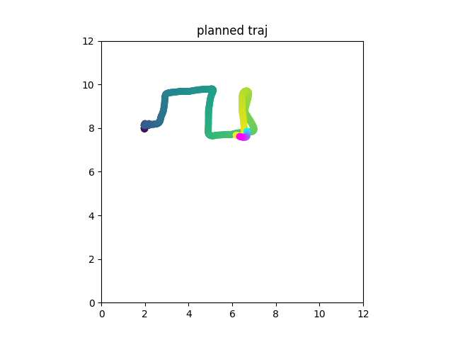
Planning with Diffusion Forcing
Diffusion Planning
Diffusion Planning
Diffusion Forcing
Why is this bad
Now you are at \(o_t\). You want an action. The best you can do is to diffuse \(x_t=[o_t, a_t, r_t]\).
But you already observed \(o_t\)!
Instead
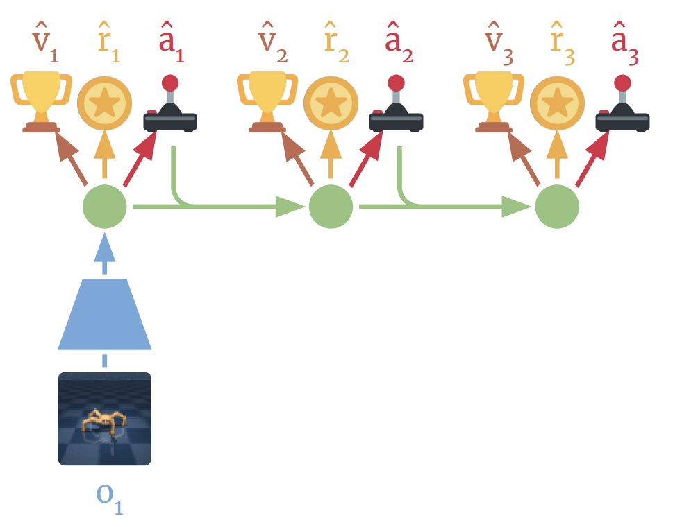
Joint distribution of policy and dynamics
After receiving ground truth \(o_{t+1}\), update posterior state by \(x_t=[o_{GT, t+1}, a_t, r_t]\)
Now we learn the distribution of data
How to get good policy instead of copying suboptimal policy?
Classifier guidance
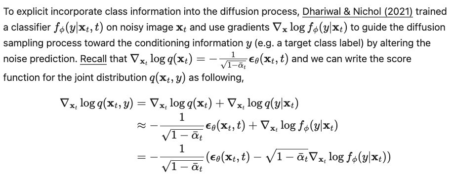
Classifier guidance
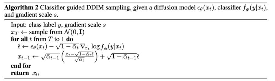
Classifier guidance
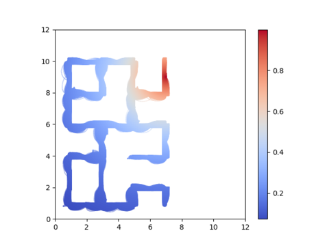
Value guidance
Define probability of task success as
\(\exp(V-V^*)\) where \(V^*\) denotes max possible value
...
Take \(V = r_t + r_{t+1} ... + r_{T}\), do value guidance
You can take \(V = r_t + r_{t+1} ... + r_{T}\) for guidance
But you can also take \(V = r_t\) for guidance
unlike previous methods
Diffusion Forcing is ANY horizon
This doesn't work immediately!
Repeated Sampling
...
x 10 samples
x 10 samples
x 10 samples
x 10 samples
Take \(V = avg(r_t + r_{t+1} ... + r_{T})\), do value guidance
This doesn't work immediately!
Why does this happen?
Why does this happen?
Perturb beginning of trajectory a bit changes later trajectory by a lot
Change \([o_{t+1}, a_t, r_t]\) should make \([o_{t+1}, a_t, r_t]\) more uncertain
While \(Noisy([o_{t+2}, a_{t+1}, r_{t+1}])\) asks it to be certain
Previous sampling
Diffusion
Step (k)
Time step (t)
N
Denote N=most noisy
N
N
N
N
N
N-1
N-1
N-1
N-1
N-1
N-1
N-2
N-2
N-2
N-2
N-2
N-2
Pyramid sampling
N
N
N
N
N
N
N-1
N-2
N
N
N
N
N
N-1
N
N
N
N
No gradient!
Pyramid sampling
Calculate guidance gradient without pyramid sampling but resample to higher noise level by adding noise
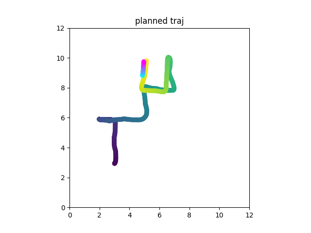
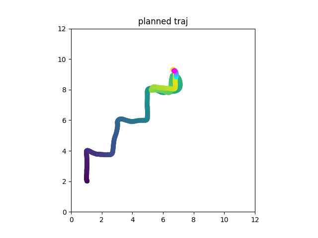
Result
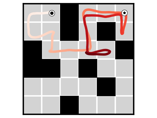
Result
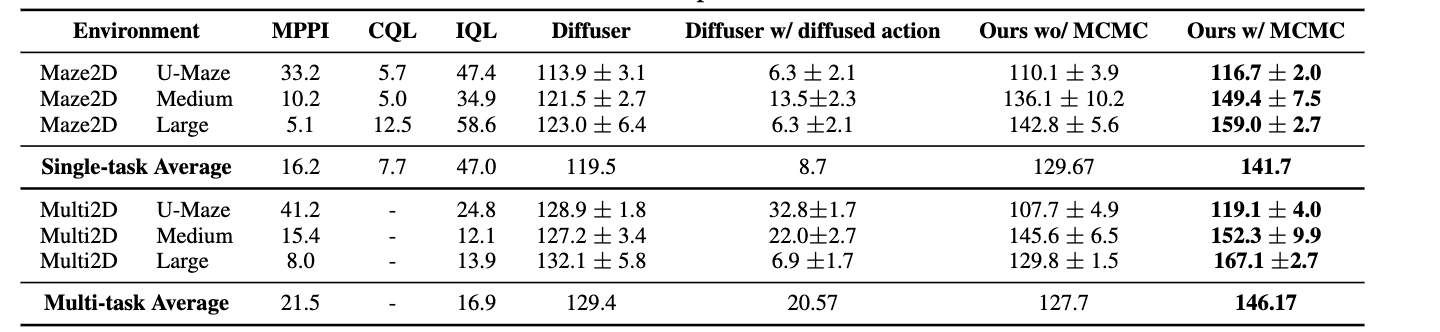
Result
Real Robot
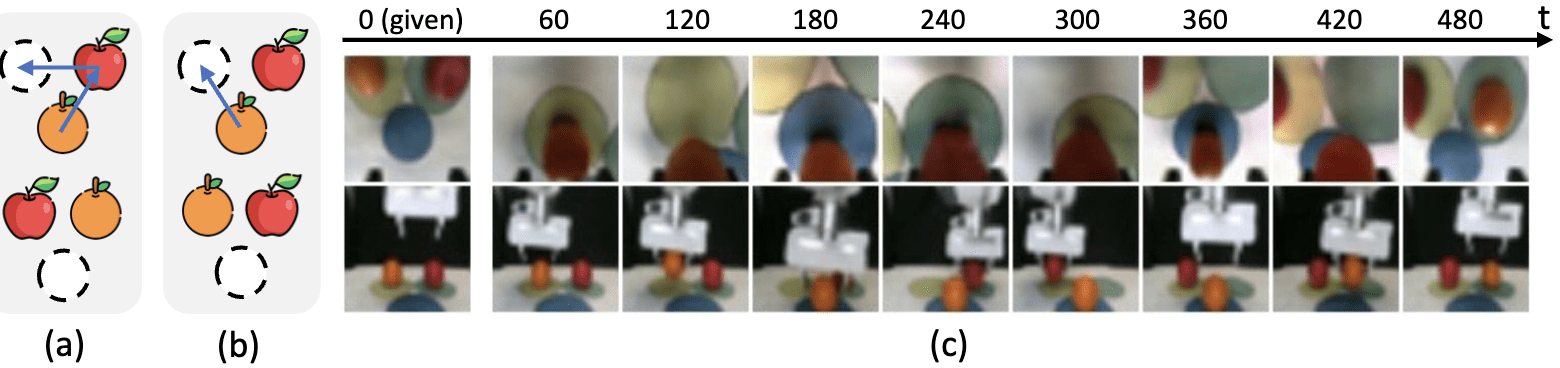
Consider a table with 3 slots. An apple an an orange are at random slots upon initialization. Task is to swap them using the third slot.
This is not markovian!
Real Robot
Just do imitation learning on this, w/ or w/ memory
Diffusion Forcing can be used as diffusion policy but with flexible horizon memory
Real Robot
Real Robot
(All images shown are predicted by diffusion)
Result
Diffusion Forcing
- Flexible
- Flexible prediction horizon
- Flexible memory horizon
- Can we auto-regressive / full sequence diffusion at user's choice without retraining
- Easy to incorporate up-coming observation
- Efficient to do MCTS over
- Guidance
- Guidance with consideration of causal uncertainty
- Guidance over longer horizon