Lab Exercise 1: What is the Most Beautiful Spot in Lake County?

We start, as always, by opening ArcMap.   The DEM we have downloaded for Lake County came in four pieces, so we need to mosaic them together with Data Management Tools >> Raster >> Raster Dataset >> Mosaic.  We put all but one of our DEM files as input and choose the one we left out as the one to which we want to mosaic the others.

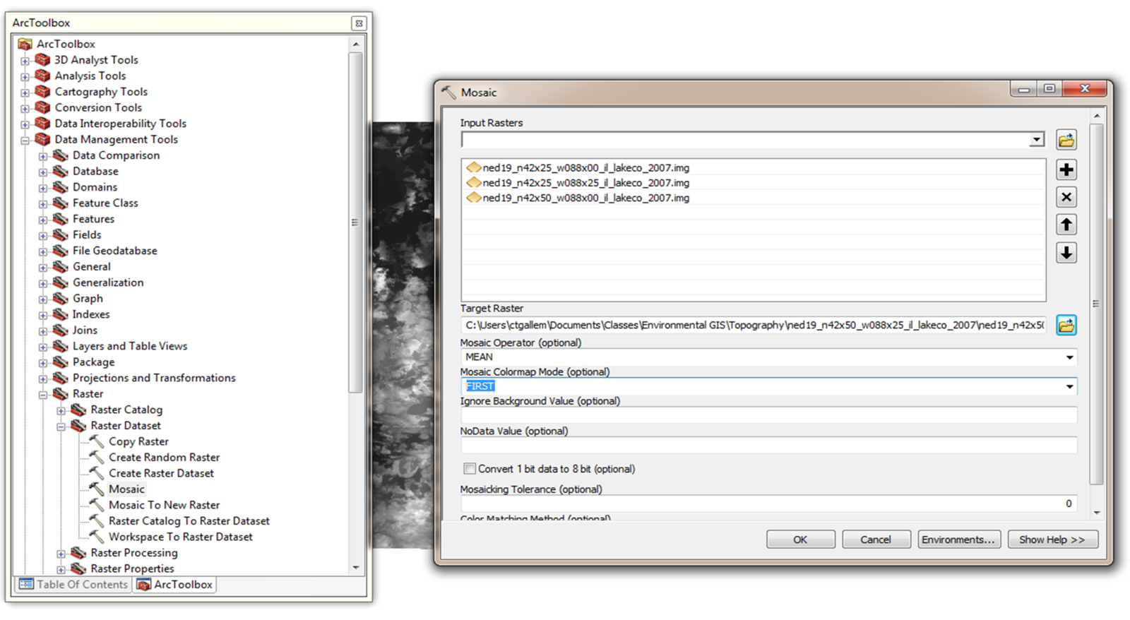
Once we've got a single raster, we need to project it into a meaningful projection (like UTM) if we are to do any topographic analysis properly.  We must have a projected DEM to be confident in topographic models.  So we go Data Management Tools >> Projections and Transformations >> Raster >> Project Raster

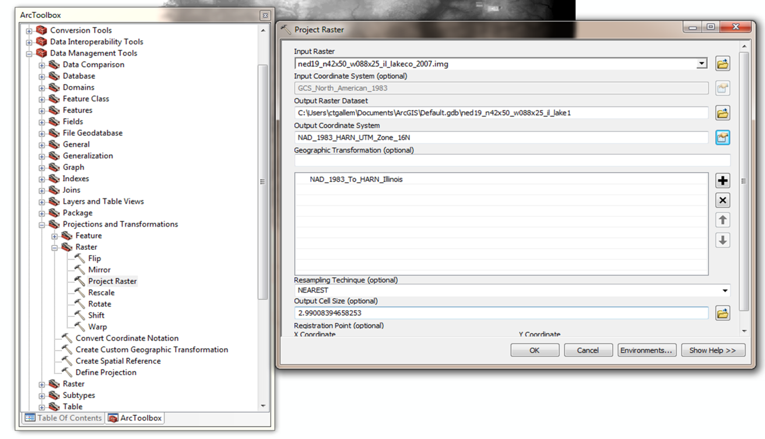
Once we have reprojected the raster, we are ready to do all kinds of analysis.  Aspect models the direction each pixel faces, in decimal degrees from true north.  It is found in Spatial Analyst Tools >> Surface >> Aspect.   The tool is pretty simple - just tell it what raster to use.

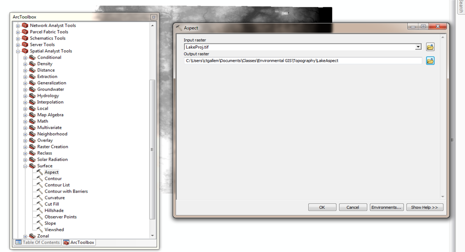
So how do we interpret this ugly output?

Our next fun one is Hillshade, which simulates shadows cast by a light like the sun.  It's not really useful for analysis, but can be used to add depth to maps.  It is also pretty simple . . . you add in the DEM and set the location of the light source.  Find this tool at Toolbox >> Spatial Analyst Tools >> Surface >> Hillshade

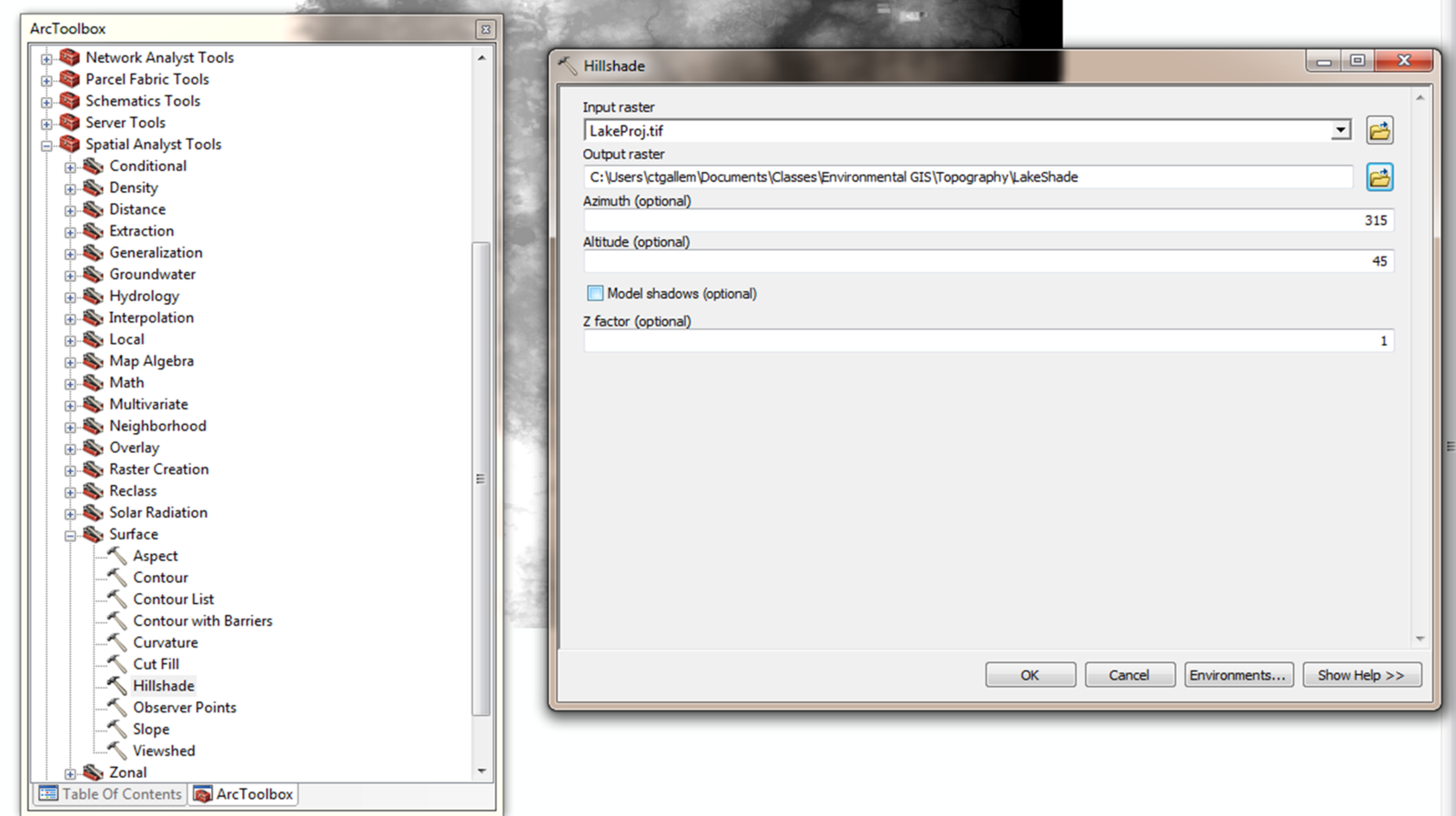
Once you make the hillshade layer, you can set it on top of the drawing order, make it semi-transparent, and then adjust the color ramp of the DEM to make a fancy-looking elevation image.

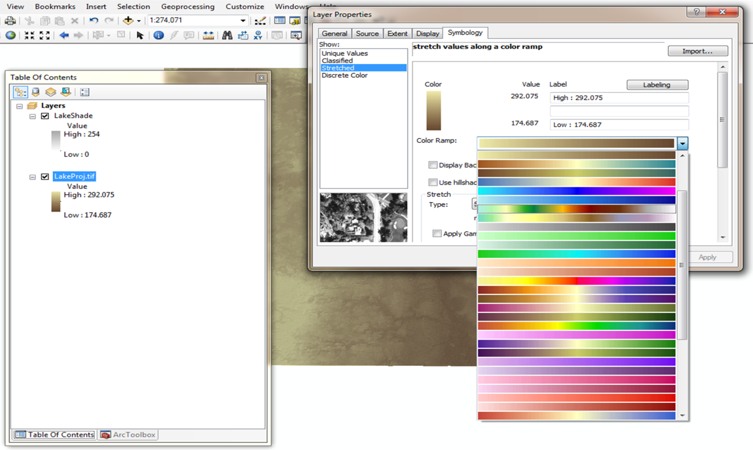
Create an image you like and add a Lab Journal Entry.

To add definition, we can also draw contour lines, with Toolbox >> Spatial Analyst Tools >> Surface >> Contour.  You have to set the intervals (i.e. how far apart will each contour line be?)

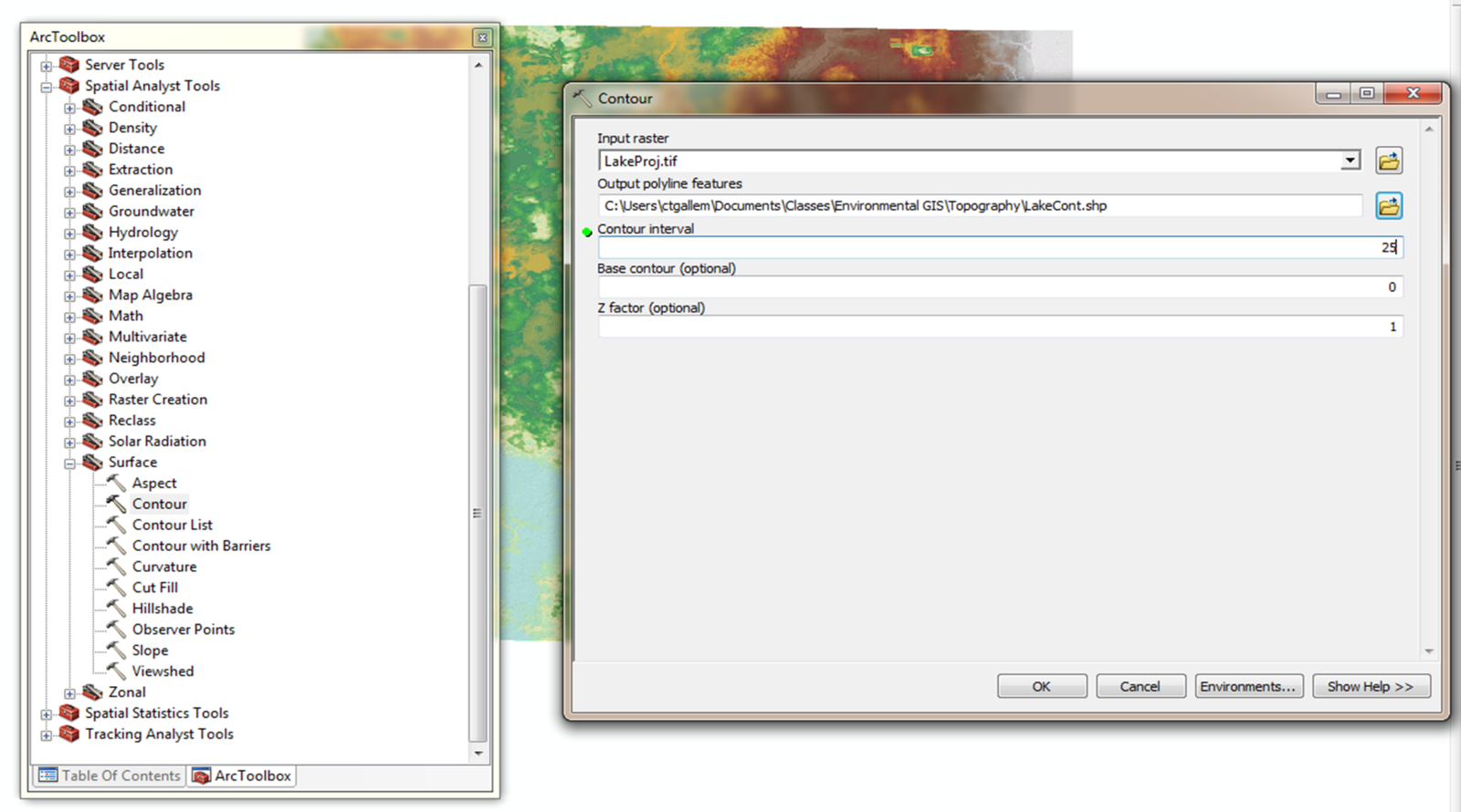
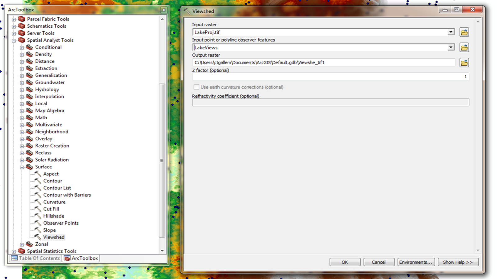
And, finally, viewshed: this takes an input point layer and determines what areas of a surface would be visible from those points.  If the resolution is any good at all it tends to be really computationally intensive, so we'll just use the one point found in the LakeViews shapefile.  If you want, you can use the editor toolbar to move the point around.

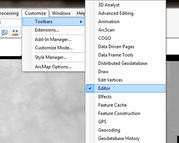
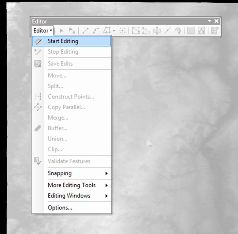
Here's how you get to the Editor toolbar.

Then choose Start Editing and you can click and drag the point wherever you want.

Add a Lab Journal entry.

That might be taking too long for us, or maybe we want to look at multiple viewpoints.  If we can get away with it, maybe we want to aggregate our DEM to make things easier.  We find it in Spatial Analyst >> Generalization >> Aggregate.

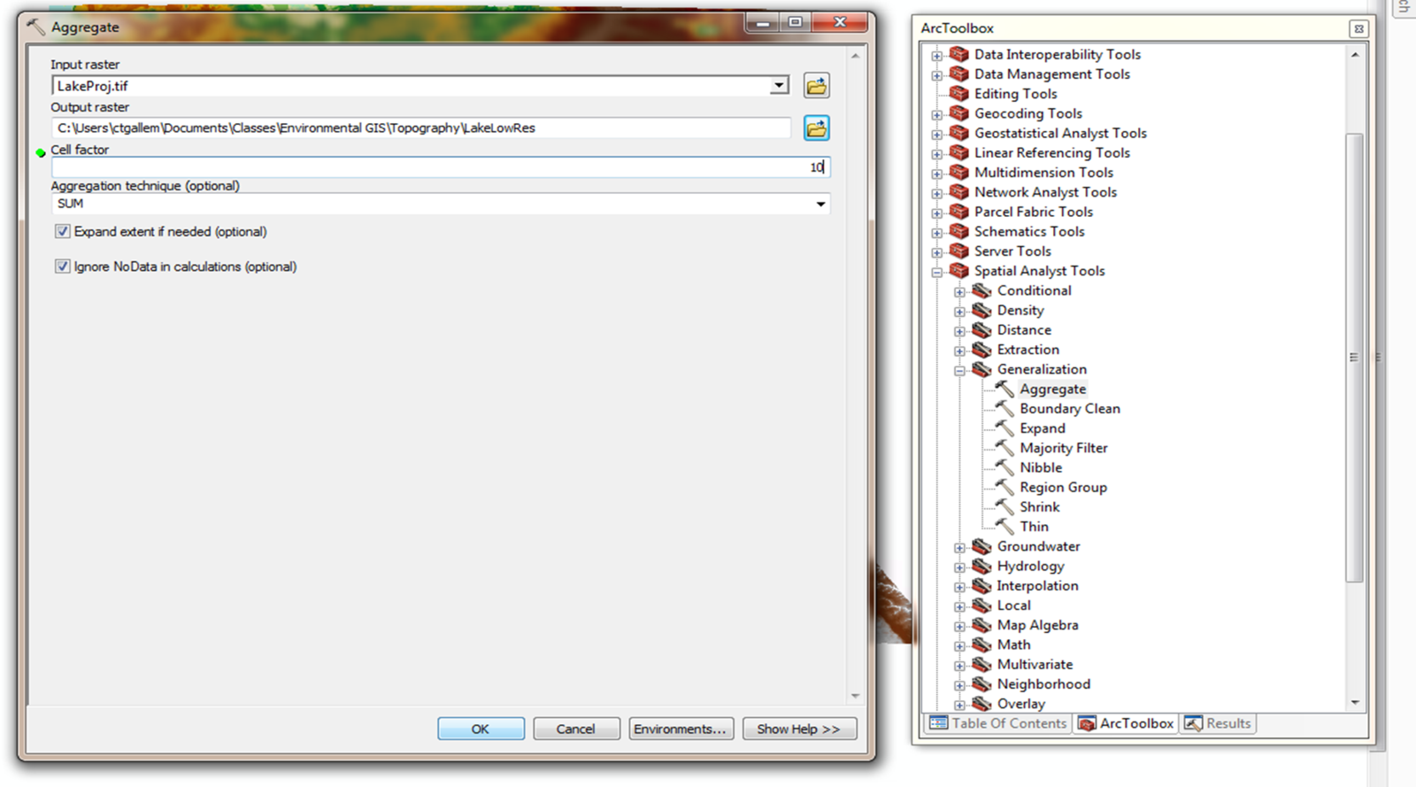
What type of Aggregation Function do we want to use?  When might we use the other functions?

Now let's see what you can see from that point.  All we have to do is run Tabulate Areas with your viewshed output as the zones and your lcproject raster as your class data:

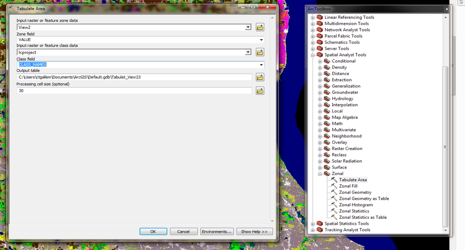
Add a Lab Journal Entry.

Lab Exercise 2: LIDAR Data and ArcScene

The LiDAR data we will be using comes from a free government dataset collected in Grand Teton National Park.  We're only using a very, very, very small section of the entire dataset, but this already consists of around 2 million points.

Remember, LiDAR data tend to come in either .las or .ascii files formats.  We're using data in a .las format.  We need a special tool in ArcMap to read these files in, so make sure that both 3-D Analyst and Spatial Analyst extensions are enabled.

First, we need to get some information about the file.  We go 3D Analyst >> Conversion >> From File >> Point File Information:

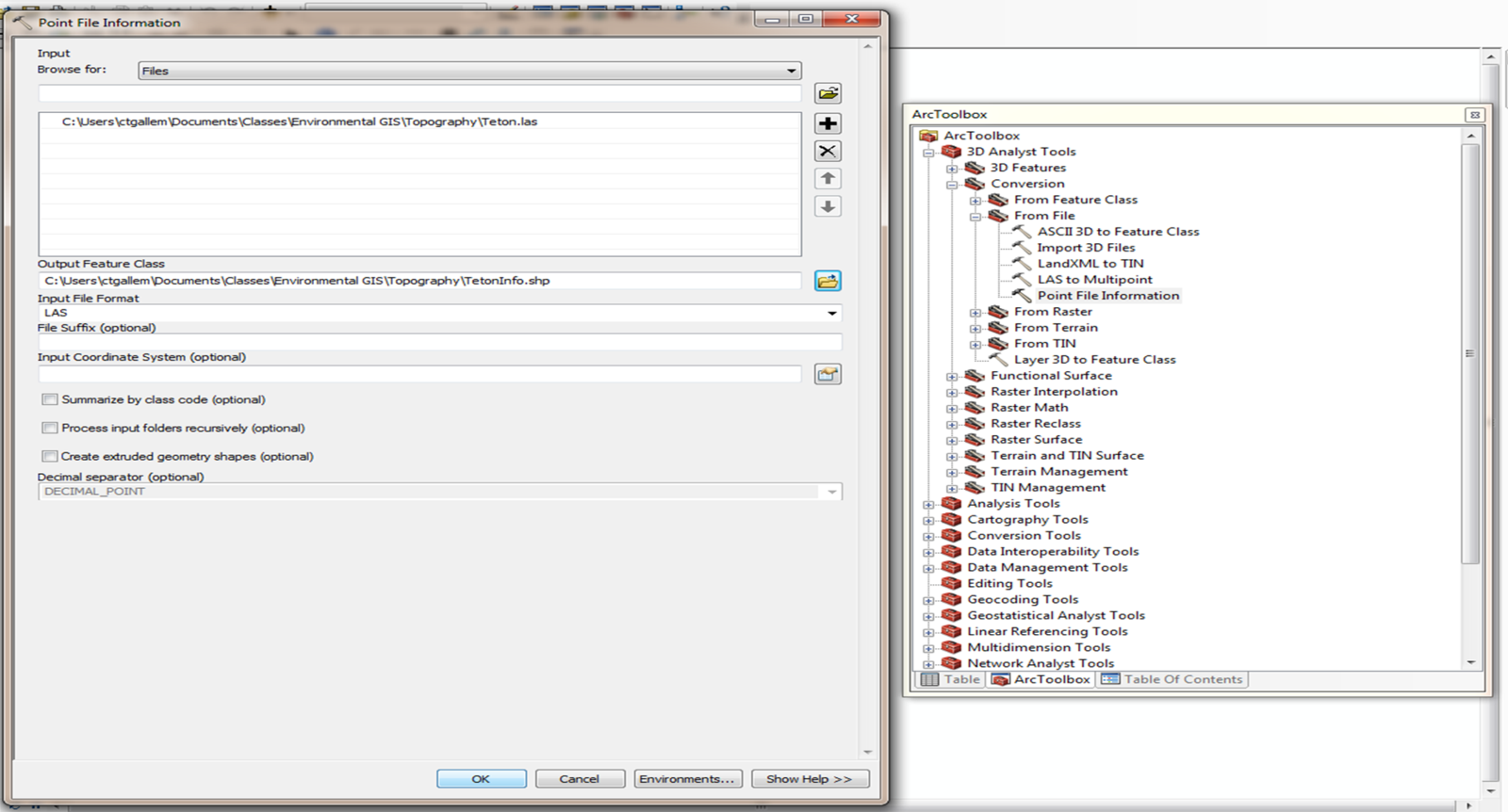
Now we can import the LAS file by going 3D Analyst >> From File >> LAS to Multipoint.  Be sure to add in that Average Point Spacing from the previous slide.

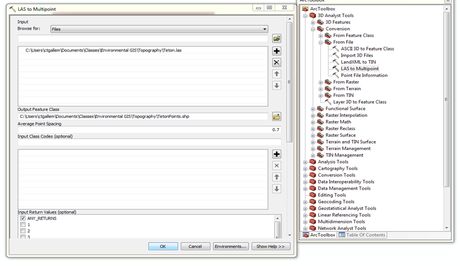
Take a Moment to look around this new Layer and Add a lab journal Entry

Triangulated Irregular Networks (TINs)

Generating a TIN is pretty simple.  Go 3D Analyst >> TIN Management >> Create TIN.  Use your LiDAR layer as your Input Feature Layer.

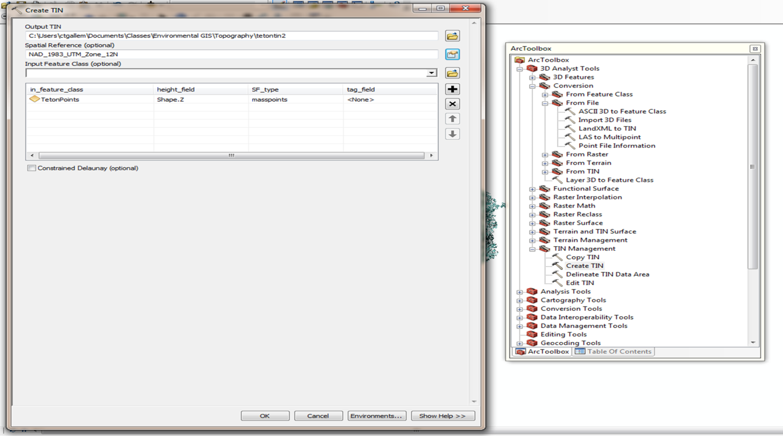
Look around at the TIN a bit.  What does it look like?  What could you do with it?

Close out arcmap and open arcscene

Let's start visualizing our DEM in ArcScence.  First, add the DEM to the scene:

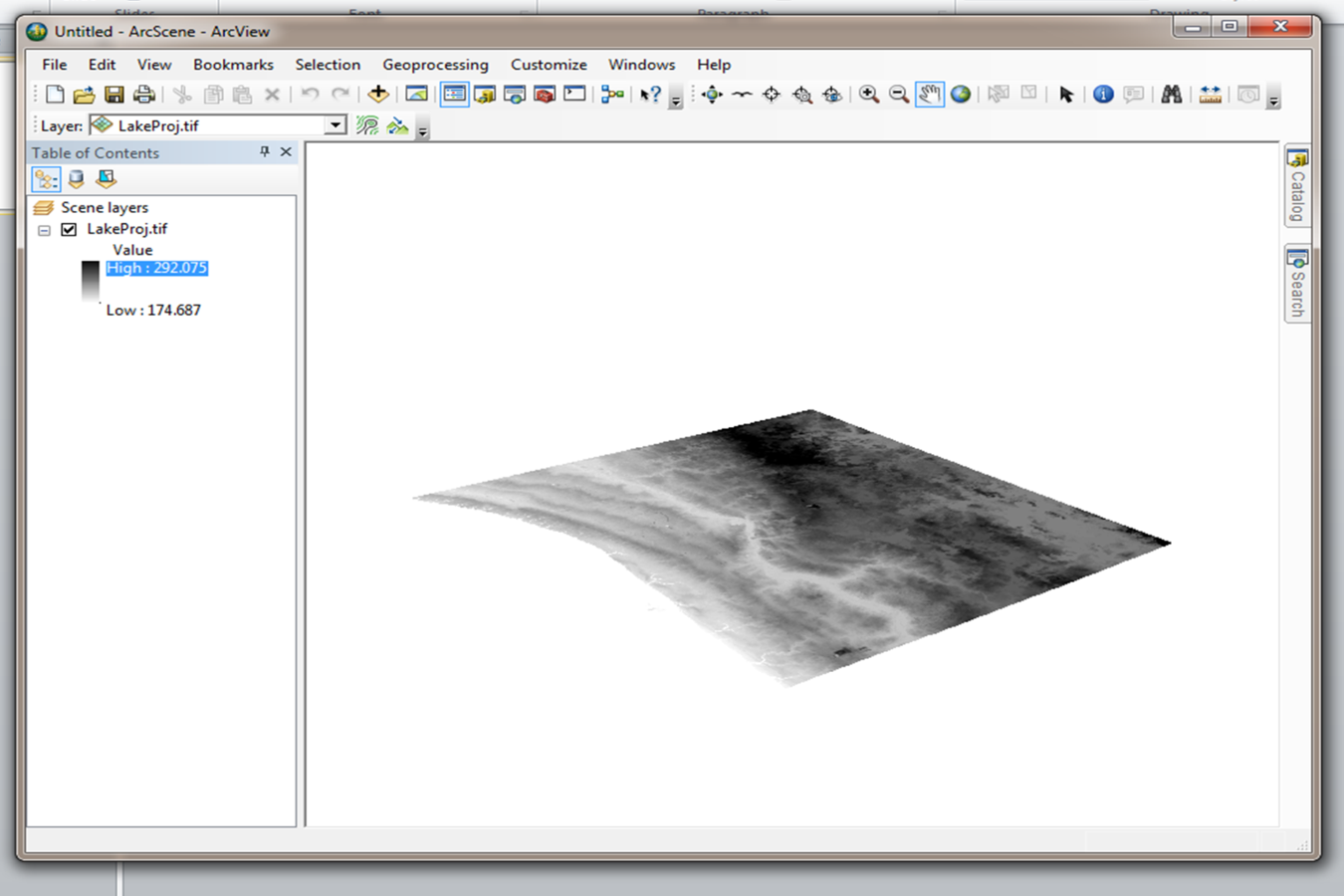
Take a Moment to Familiarize yourself with the Navigation in ArcScene.  It can be a little tricky.

So our DEM is looking a little flat.  Let's fix that.  All we need to do is right click on the DEM layer, choose Properties, and set the Base Height so that the heights will reflect the elevation of the DEM pixels.  Choose "Floating on a custom surface" and pick the DEM as that surface.

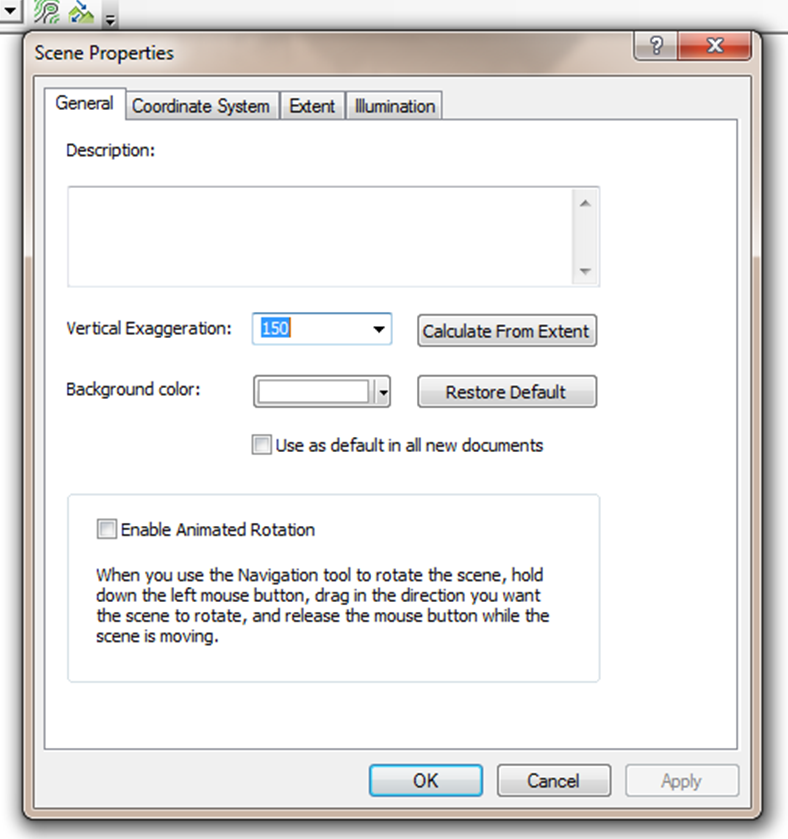
This still might not be enough.  To see a difference, we might need to right-click on our scene in the table of contents, select Properties, open the General tab and manipulate our Vertical Exaggeration until we're happy:

Now let's get fancy.  Let's add the hillshade in, go to properties, and then set it to have the same elevation of our DEM:

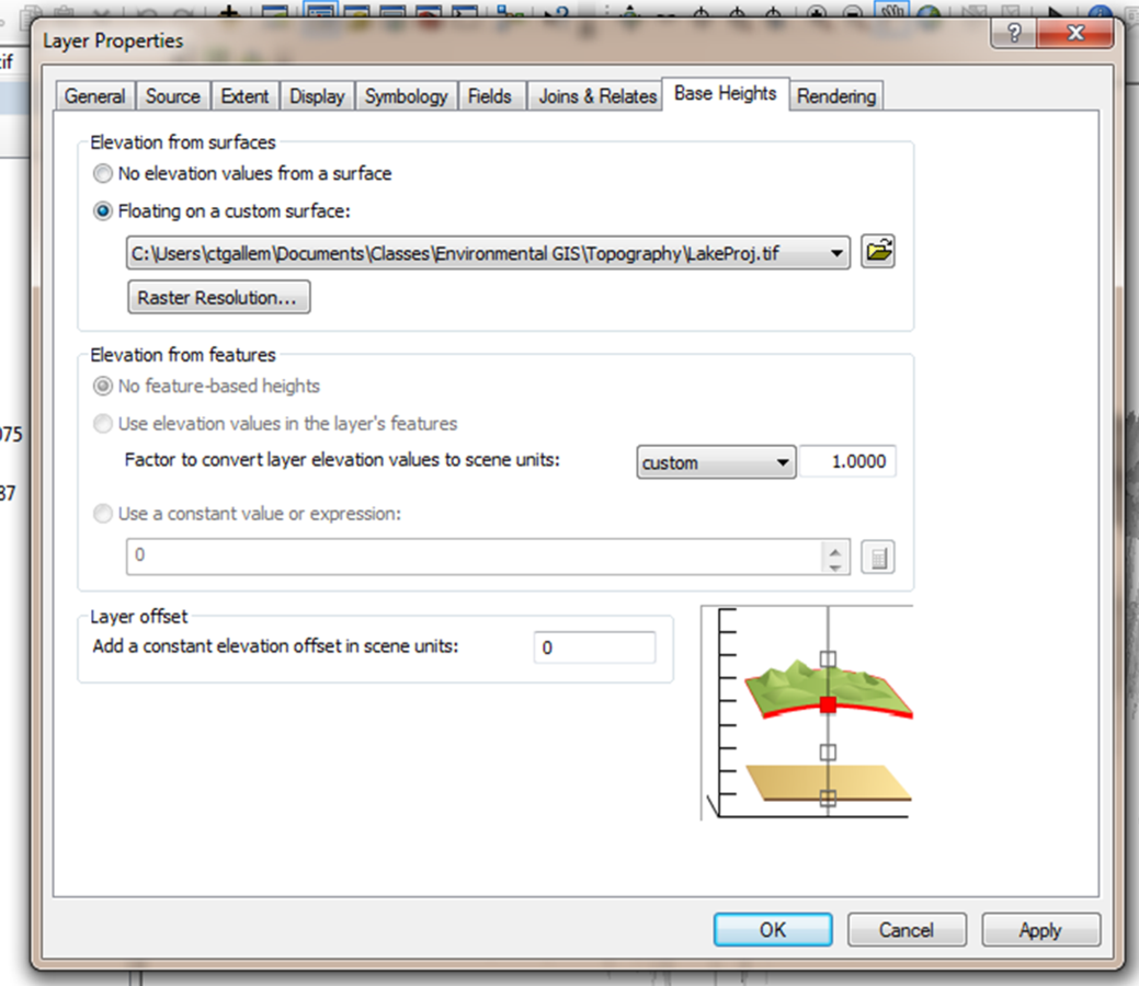
Add a Lab journal entry.

Start a New Scene in ArcScene.

Okay, now for the really hard part: visualizing a TIN in ArcScene.  Add your TIN to your new scene in ArcScene:

Oh, actually, that's about it.  You Have successfully visualized a TIN in ArcScene!  Add a lab journal entry.