神經網路
講師:溫室蔡
機器學習[2]
神經網路結構
?
多層感知器(mLP)
隱藏層
輸入層
輸出層
權重
權重
感知器數學
x_1
x_2
x_3
z_1=w_1x_1+w_2x_2+w_3x_3+b_1
w_1
w_2
w_3
b_1
向量加法、內積
\mathbf{a}=
\begin{bmatrix}
a_1\\a_2\\a_3\\
\end{bmatrix},
\mathbf{b}=
\begin{bmatrix}
b_1\\b_2\\b_3\\
\end{bmatrix}
\mathbf{a}\cdot\mathbf{b}=
a_1b_1+a_2b_2+a_3b_3
\mathbf{a}+\mathbf{b}=
\begin{bmatrix}
a_1+b_1\\a_2+b_2\\a_3+b_3\\
\end{bmatrix}
感知器數學
x_1
x_2
x_3
z_1=w_1x_1+w_2x_2+w_3x_3+b_1
w_1
w_2
w_3
b_1
感知器數學
x_1
x_2
x_3
z_1=\mathbf{w}\cdot\mathbf{x}+b_1
w_1
w_2
w_3
b_1
\mathbf{w}=
\begin{bmatrix}
w_1\\w_2\\w_3\\
\end{bmatrix},
\mathbf{x}=
\begin{bmatrix}
x_1\\x_2\\x_3\\
\end{bmatrix}
再一個感知器
x_1
x_2
x_3
z_1
b_1
再一個感知器
x_1
x_2
x_3
z_1
b_1
z_2
b_2
再一個感知器
x_1
x_2
x_3
z_1
b_1
z_2
b_2
w_{11}
w_{12}
w_{13}
w_{21}
w_{22}
w_{23}
再一個感知器
x_1
x_2
x_3
z_1=w_{11}x_1+w_{12}x_2+w_{13}x_3+b_1
b_1
z_2=w_{21}x_1+w_{22}x_2+w_{23}x_3+b_2
b_2
w_{11}
w_{12}
w_{13}
w_{21}
w_{22}
w_{23}
矩陣乘法
\mathbf{A}=
\begin{bmatrix}
a_{11}&a_{12}&a_{13}\\
a_{21}&a_{22}&a_{23}\\
\end{bmatrix}
\mathbf{x}=
\begin{bmatrix}
x_1\\x_2\\x_3\\
\end{bmatrix}
矩陣乘法
y_1=a_{11}x_1+a_{12}x_2+a_{13}x_3
y_2=a_{21}x_1+a_{22}x_2+a_{23}x_3
\mathbf{A}\mathbf{x}=\mathbf{y}=
\begin{bmatrix}
y_1\\y_2
\end{bmatrix}
矩陣乘法
\begin{bmatrix}
a_{11}&a_{12}&a_{13}\\
a_{21}&a_{22}&a_{23}\\
\end{bmatrix}
\begin{bmatrix}
x_1\\x_2\\x_3\\
\end{bmatrix}
\begin{bmatrix}
y_1\\y_2\\
\end{bmatrix}
矩陣乘法
\begin{bmatrix}
a_{11}&a_{12}&a_{13}\\
a_{21}&a_{22}&a_{23}\\
\end{bmatrix}
\begin{bmatrix}
x_1\\x_2\\x_3\\
\end{bmatrix}
\begin{bmatrix}
y_1\\y_2\\
\end{bmatrix}
矩陣乘法
\begin{bmatrix}
a_{11}&a_{12}&a_{13}\\
a_{21}&a_{22}&a_{23}\\
\end{bmatrix}
\begin{bmatrix}
x_1\\x_2\\x_3\\
\end{bmatrix}
\begin{bmatrix}
y_1\\y_2\\
\end{bmatrix}
線代化
x_1
x_2
x_3
b_1
z_2=w_{21}x_1+w_{22}x_2+w_{23}x_3+b_2
b_2
w_{11}
w_{12}
w_{13}
w_{21}
w_{22}
w_{23}
z_1=w_{11}x_1+w_{12}x_2+w_{13}x_3+b_1
線代化
x_1
x_2
x_3
\mathbf{z}=\mathbf{W}\mathbf{x}+\mathbf{b}
b_1
b_2
w_{11}
w_{12}
w_{13}
w_{21}
w_{22}
w_{23}
\mathbf{x}=
\begin{bmatrix}
x_1\\x_2\\x_3
\end{bmatrix},
\mathbf{W}=
\begin{bmatrix}
w_{11}&w_{12}&w_{13}\\
w_{21}&w_{22}&w_{23}
\end{bmatrix},
\mathbf{b}=
\begin{bmatrix}
b_1\\b_2
\end{bmatrix},
\mathbf{z}=
\begin{bmatrix}
z_1\\z_2
\end{bmatrix}
z_2
z_1
前向傳播
\mathbf{W}_1
\mathbf{W}_2
\mathbf{x}_0
\mathbf{x}_1=\mathbf{W}_1\mathbf{x}_0+\mathbf{b}_1
\mathbf{x}_2=\mathbf{W}_2\mathbf{x}_1+\mathbf{b}_2
退化
\mathbf{x}_1=\mathbf{W}_1\mathbf{x}_0+\mathbf{b}_1
\mathbf{x}_2=\mathbf{W}_2\mathbf{x}_1+\mathbf{b}_2
退化
\Bigg\Downarrow
代入
\mathbf{x}_1=\mathbf{W}_1\mathbf{x}_0+\mathbf{b}_1
\mathbf{x}_2=\mathbf{W}_2\mathbf{x}_1+\mathbf{b}_2
退化
\mathbf{x}_2=\mathbf{W}_2(\mathbf{W}_1\mathbf{x}_0+\mathbf{b}_1)+\mathbf{b}_2
\Bigg\Downarrow
代入
\mathbf{x}_1=\mathbf{W}_1\mathbf{x}_0+\mathbf{b}_1
退化
\mathbf{x}_2=(\mathbf{W}_2\mathbf{W}_1)\mathbf{x}_0+(\mathbf{W}_2\mathbf{b}_1+\mathbf{b}_2)
雖然經過了多層的變換
最後一層與第一層卻依然是線性關係
依然是線性分類器
激勵函數
在前向傳播中加入一些非線性的函數
前向傳播
\mathbf{W}_1
\mathbf{W}_2
\mathbf{x}_0
\mathbf{x}_1=\sigma(\mathbf{W}_1\mathbf{x}_0+\mathbf{b}_1)
\mathbf{x}_2=\sigma(\mathbf{W}_2\mathbf{x}_1+\mathbf{b}_2)
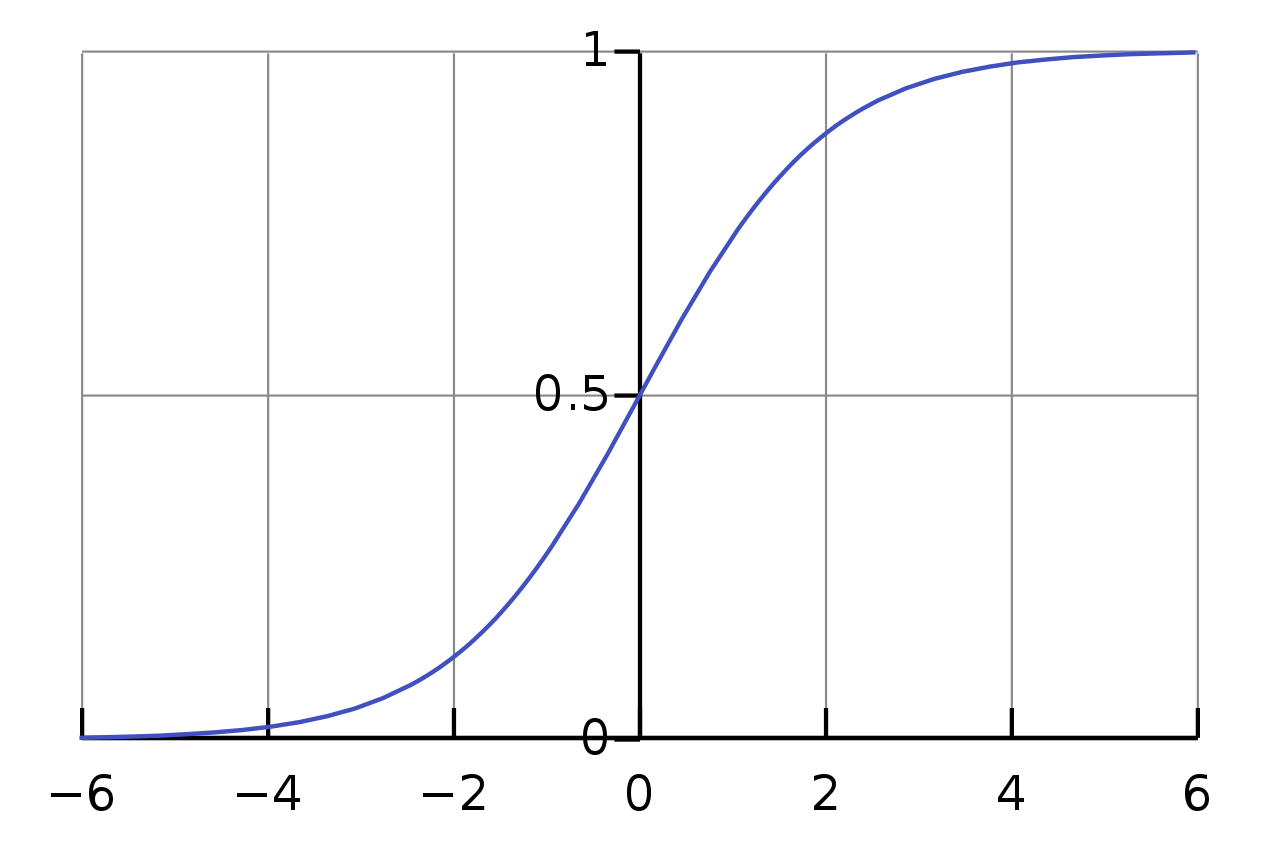
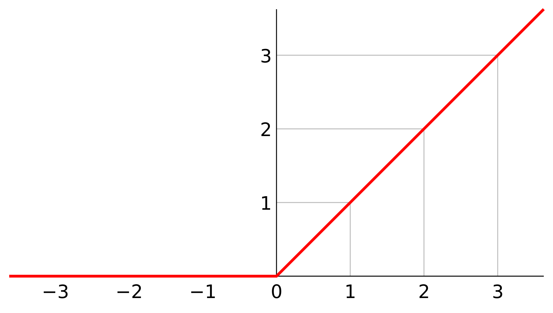
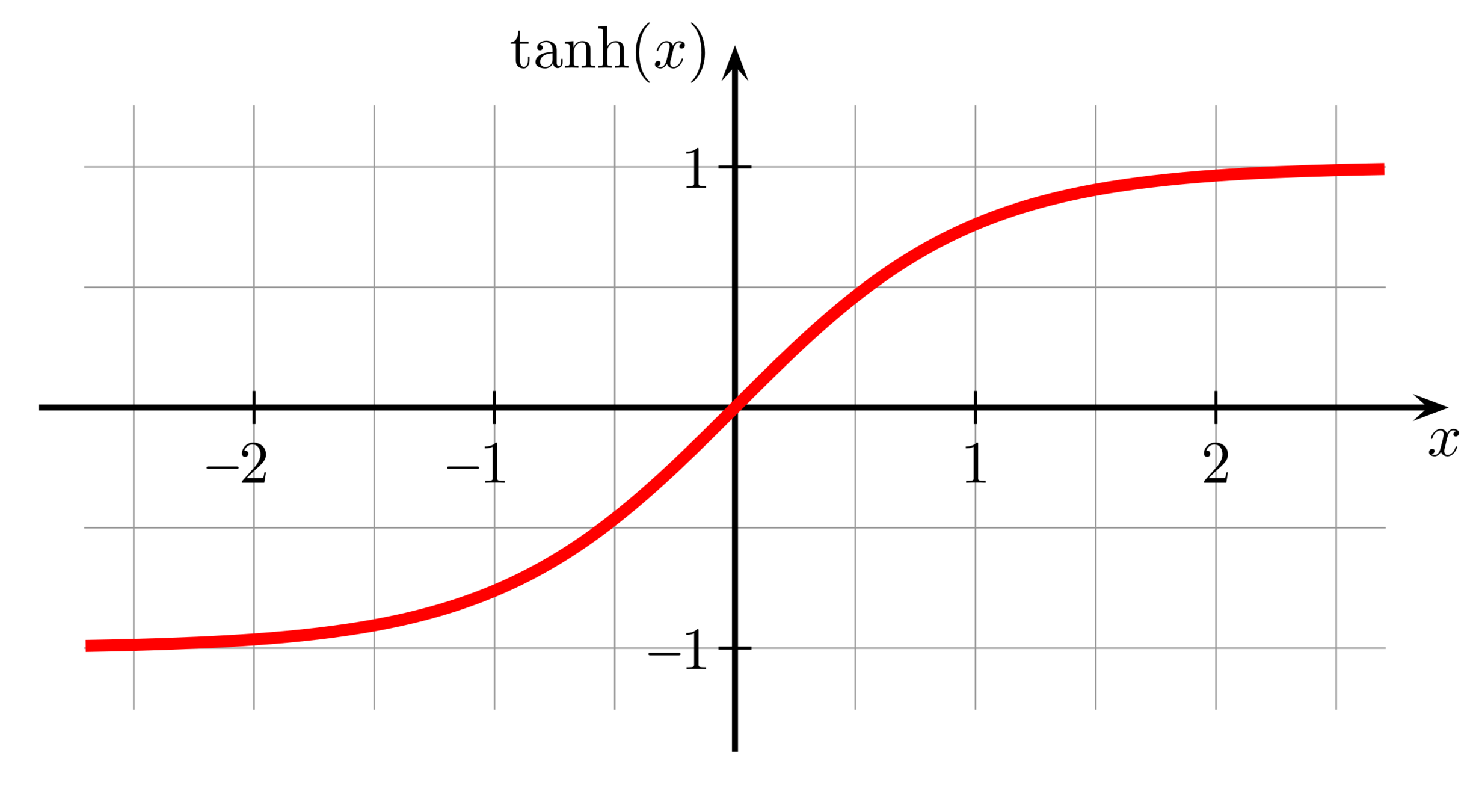
常見的激勵函數
\sigma(x)=\dfrac{1}{1+e^{-x}}
\tanh(x)=\dfrac{e^x-e^{-x}}{e^x+e^{-x}}
\mathrm{ReLU}(x)=\max(0, x)
損失函數
\mathbf{W}_1
\mathbf{W}_2
\mathbf{x}_0
\mathbf{x}_1
\mathbf{x}_2
\mathbf{y}
輸入
輸出
正解
\mathcal{L}=(\mathbf{x}_2-\mathbf{y})^2
差異
梯度下降
我們沒辦法直接求得損失函數的最小值
但我們可以從函數圖形的角度去思考
求出「目前參數下,損失函數圖形的梯度」
然後將參數往梯度反方向更新
就可以在損失函數圖形上往下坡走
梯度下降
損失
參數
梯度下降
損失
參數
梯度下降
損失
參數
梯度下降
損失
參數
梯度下降
(\mathbf{W},\mathbf{b})_{t+1}=(\mathbf{W},\mathbf{b})_t-\gamma\nabla\mathcal{L}
梯度下降可以用以下的數學式描述:
更新後參數
目前參數
學習率
(下降步長)
損失函數梯度
微分
y
x
\Delta x
\Delta y
函數圖形在某點的斜率
\approx\dfrac{\Delta y}{\Delta x}
微分
y
x
\Delta x
\Delta y
函數圖形在某點的斜率
\approx\dfrac{\Delta y}{\Delta x}
=\displaystyle\lim_{\Delta x \rightarrow 0}\dfrac{\Delta y}{\Delta x}
微分
y
x
\mathrm dx
\mathrm dy
函數圖形在某點的斜率
\approx\dfrac{\Delta y}{\Delta x}
=\displaystyle\lim_{\Delta x \rightarrow 0}\dfrac{\Delta y}{\Delta x}
=\dfrac{\mathrm dy}{\mathrm dx}
微分操作-定義法
計算微分的一種方法
f'(x)=\displaystyle\lim_{\Delta x\rightarrow0}\dfrac{f(x+\Delta x)-f(x)}{\Delta x}
是直接從微分的定義做起
註:
f'(x)
是
\dfrac{\mathrm df}{\mathrm dx}
的簡便寫法
微分操作-定義法
f(x)=x^3
\begin{aligned}
f'(x)
&=\displaystyle\lim_{\Delta x\rightarrow0}\dfrac{(x+\Delta x)^3-x^3}{\Delta x}\\
&=\displaystyle\lim_{\Delta x\rightarrow0}\dfrac{x^3+3x^2\Delta x+3x(\Delta x)^2+(\Delta x)^3-x^3}{\Delta x}\\
&=\displaystyle\lim_{\Delta x\rightarrow0}3x^2+3x\Delta x+(\Delta x)^2\\
&=3x^2
\end{aligned}
微分操作-規則法
所以實務上是直接記住微分的規則
直接從定義做會很麻煩
然後照這些規則去計算
微分規則
次方律:
\dfrac{\mathrm d(x^n)}{\mathrm dx}=nx^{n-1}
加法律:
\dfrac{\mathrm d(f+g)}{\mathrm dx}=\dfrac{\mathrm df}{\mathrm dx}+\dfrac{\mathrm dg}{\mathrm dx}
乘法律:
\dfrac{\mathrm d(fg)}{\mathrm dx}=\dfrac{\mathrm df}{\mathrm dx}g+f\dfrac{\mathrm dg}{\mathrm dx}
連鎖律:
\dfrac{\mathrm d(f(g(x)))}{\mathrm dx}=\dfrac{\mathrm df}{\mathrm dg}\dfrac{\mathrm dg}{\mathrm dx}
指數微分
\dfrac{\mathrm d(e^x)}{\mathrm dx}=e^x
\begin{aligned}
\dfrac{\mathrm d(a^x)}{\mathrm dx}
&=\dfrac{\mathrm d((e^{\ln a})^x)}{\mathrm dx}\\
&=\dfrac{\mathrm d(e^{x \ln a})}{\mathrm dx}\\
&=\dfrac{\mathrm d(e^{x \ln a})}{\mathrm d(x \ln a)}\dfrac{\mathrm d(x \ln a)}{\mathrm dx}\\
&=e^{x \ln a}\ln a\\
&=a^x\ln a\\
\end{aligned}
對數微分
\begin{aligned}
& y=\ln x\\
& \Rightarrow e^y=x\\
& \Rightarrow \mathrm d(e^y)=\mathrm dx\\
& \Rightarrow \dfrac{\mathrm d(e^y)}{\mathrm dy}\mathrm dy=\mathrm dx\\
& \Rightarrow e^y\mathrm dy=\mathrm dx\\
& \Rightarrow \dfrac{\mathrm dy}{\mathrm dx}=\dfrac{1}{e^y}=\dfrac{1}{x}
\end{aligned}
三角函數微分
\sin x
-\sin x
-\cos x
\cos x
\Longrightarrow
微分
\Big\Downarrow
微分
\Longleftarrow
微分
\Big\Uparrow
微分
\mathbf{W}_1
\mathbf{W}_2
\mathbf{x}_0
\mathbf{x}_1
\mathbf{x}_2
\mathbf{y}
輸入
輸出
正解
\mathcal{L}=(\mathbf{x}_2-\mathbf{y})^2
差異
對損失函數微分
對損失函數微分
\mathbf W_\ell
\mathbf{x}_{\ell-1}
\mathbf{x}_\ell
\mathbf{y}
輸出
正解
\mathcal{L}=(\mathbf{x}_\ell-\mathbf{y})^2
差異
對損失函數微分
\mathcal{L}=(\mathbf{x}_\ell-\mathbf{y})^2
對損失函數微分
\mathbf{x}_\ell=\sigma(\mathbf W_\ell \mathbf{x}_{\ell-1}+\mathbf b_\ell)
\mathcal{L}=(\mathbf{x}_\ell-\mathbf{y})^2
對損失函數微分
\mathcal{L}=(\mathbf{x}_\ell-\mathbf{y})^2
\mathbf{x}_\ell=\sigma(\mathbf z_\ell)
\mathbf{z}_\ell=\mathbf W_\ell \mathbf{x}_{\ell-1}+\mathbf b_\ell
對損失函數微分
\dfrac{\partial \mathcal{L}}{\partial \mathbf W_\ell}=
\dfrac{\partial \mathcal{L}}{\partial \mathbf x_\ell}
\dfrac{\partial \mathbf x_\ell}{\partial \mathbf z_\ell}
\dfrac{\partial \mathbf z_\ell}{\partial \mathbf W_\ell}
\mathcal{L}=(\mathbf{x}_\ell-\mathbf{y})^2
\mathbf{x}_\ell=\sigma(\mathbf z_\ell)
\mathbf{z}_\ell=\mathbf W_\ell \mathbf{x}_{\ell-1}+\mathbf b_\ell
對損失函數微分
\begin{aligned}
\dfrac{\partial \mathcal{L}}{\partial \mathbf W_\ell}
&=
\dfrac{\partial \mathcal{L}}{\partial \mathbf x_\ell}
\dfrac{\partial \mathbf x_\ell}{\partial \mathbf z_\ell}
\dfrac{\partial \mathbf z_\ell}{\partial \mathbf W_\ell}
\\
&=2(\mathbf x_\ell-\mathbf{y})\sigma'(\mathbf z_\ell)\mathbf{x}_{\ell-1}
\end{aligned}
\mathcal{L}=(\mathbf{x}_\ell-\mathbf{y})^2
\mathbf{x}_\ell=\sigma(\mathbf z_\ell)
\mathbf{z}_\ell=\mathbf W_\ell \mathbf{x}_{\ell-1}+\mathbf b_\ell
對損失函數微分
\mathcal{L}=(\mathbf{x}_\ell-\mathbf{y})^2
\mathbf{z}_\ell=\mathbf W_\ell \mathbf{x}_{\ell-1}+\mathbf b_\ell
\mathbf{x}_\ell=\sigma(\mathbf z_\ell)
\begin{aligned}
\dfrac{\partial \mathcal{L}}{\partial \mathbf b_\ell}
&=
\dfrac{\partial \mathcal{L}}{\partial \mathbf x_\ell}
\dfrac{\partial \mathbf x_\ell}{\partial \mathbf z_\ell}
\dfrac{\partial \mathbf z_\ell}{\partial \mathbf b_\ell}
\\
&=2(\mathbf x_\ell-\mathbf{y})\sigma'(\mathbf z_\ell)
\end{aligned}
更新參數
(\mathbf W_\ell)_{t+1} = (\mathbf W_\ell)_t - \gamma\dfrac{\partial \mathcal{L}}{\partial (\mathbf W_\ell)_t}
因此我們可得:
(\mathbf b_\ell)_{t+1} = (\mathbf b_\ell)_t - \gamma\dfrac{\partial \mathcal{L}}{\partial (\mathbf b_\ell)_t}
反向傳播
\begin{aligned}
\dfrac{\partial \mathcal{L}}{\partial \mathbf W_{\ell-1}}
&=
\dfrac{\partial \mathcal{L}}{\partial \mathbf x_{\ell-1}}
\dfrac{\partial \mathbf x_{\ell-1}}{\partial \mathbf z_{\ell-1}}
\dfrac{\partial \mathbf z_{\ell-1}}{\partial \mathbf W_{\ell-1}}
\\
&=\dfrac{\partial \mathcal{L}}{\partial \mathbf x_{\ell-1}}\sigma'(\mathbf z_{\ell-1})\mathbf x_{\ell-1}
\end{aligned}
若要更新更前面一層的權重,我們會計算
如何求得?
反向傳播
在計算上一層梯度的時候
\dfrac{\partial \mathcal{L}}{\partial \mathbf W_\ell}=
\dfrac{\partial \mathcal{L}}{\partial \mathbf x_\ell}
\dfrac{\partial \mathbf x_\ell}{\partial \mathbf z_\ell}
\dfrac{\partial \mathbf z_\ell}{\partial \mathbf W_\ell}
\dfrac{\partial \mathcal{L}}{\partial \mathbf b_\ell}=
\dfrac{\partial \mathcal{L}}{\partial \mathbf x_\ell}
\dfrac{\partial \mathbf x_\ell}{\partial \mathbf z_\ell}
\dfrac{\partial \mathbf z_\ell}{\partial \mathbf b_\ell}
就可以先計算
\dfrac{\partial \mathcal{L}}{\partial \mathbf x_{\ell-1}}=
\dfrac{\partial \mathcal{L}}{\partial \mathbf x_\ell}
\dfrac{\partial \mathbf x_\ell}{\partial \mathbf z_\ell}
\dfrac{\partial \mathbf z_\ell}{\partial \mathbf x_{\ell-1}}
反向傳播
\begin{aligned}
\dfrac{\partial \mathcal{L}}{\partial \mathbf x_{\ell-1}}
&=
\dfrac{\partial \mathcal{L}}{\partial \mathbf x_\ell}
\dfrac{\partial \mathbf x_\ell}{\partial \mathbf z_\ell}
\dfrac{\partial \mathbf z_\ell}{\partial \mathbf x_{\ell-1}}
\\
&=2(\mathbf x_\ell-\mathbf{y})\sigma'(\mathbf z_\ell)\mathbf W_\ell
\end{aligned}
\mathbf{z}_\ell=\mathbf W_\ell \mathbf{x}_{\ell-1}+\mathbf b_\ell
反向傳播
以此類推,這就是「反向傳播」的概念
層計算出 給 層使用
\ell
\dfrac{\partial \mathcal{L}}{\partial \mathbf x_{\ell-1}}
\ell-1
層再計算出 給 層使用
\ell-2
\dfrac{\partial \mathcal{L}}{\partial \mathbf x_{\ell-2}}
\ell-1
手刻神經網路
import numpy as np

class NeuralNetwork:
    def __init__(self, layer_sizes, act, dact):
        self.layer_sizes = layer_sizes
        self.num_layers = len(layer_sizes) - 1
        self.act = act
        self.dact = dact
        self.weights = []
        self.biases = []
        self.zetas = []
        self.values = []
        for i in range(self.num_layers):
            self.weights.append(np.random.randn(layer_sizes[i+1], layer_sizes[i]))
            self.biases.append(np.random.randn(layer_sizes[i+1], 1))
            self.zetas.append(np.zeros((layer_sizes[i+1], 1)))
            self.values.append(np.zeros((layer_sizes[i], 1)))
        self.values.append(np.zeros((layer_sizes[-1], 1)))

    def forward(self, data):
        self.values[0] = data
        for i in range(self.num_layers):
            self.zetas[i] = np.dot(self.weights[i], self.values[i]) + self.biases[i]
            self.values[i+1] = self.act(self.zetas[i])

    def backward(self, label, lr):
        dx = self.values[-1] - label
        for i in range(self.num_layers):
            j = self.num_layers - i - 1
            db = dx * self.dact(self.zetas[j])
            dW = np.dot(db, self.values[j].T)
            dx = np.dot(self.weights[j].T, db)
            self.weights[j] -= lr * dW
            self.biases[j] -= lr * db

    def predict(self, data):
        self.forward(data)
        return self.values[-1]

    def fit(self, data, labels, lr, epochs):
        for i in range(epochs):
            print(i)
            for j in range(len(data)):
                self.forward(data[j])
                self.backward(labels[j], lr)
XOR 測試
y
x
實作 XOR 閘
是最簡單的非線性問題
因為它的資料點
沒辦法被一條直線分類
0
1
0
1
XOR 測試
from nn import NeuralNetwork
import numpy as np

def sigmoid(x):
    return 1 / (1 + np.exp(-x))

def dsigmoid(x):
    return sigmoid(x) * (1 - sigmoid(x))

if __name__ == '__main__':
    data = np.array([[0, 0], [0, 1], [1, 0], [1, 1]]).reshape((4, 2, 1))
    labels = np.array([0, 1, 1, 0]).reshape((4, 1, 1))

    model = NeuralNetwork([2, 4, 4, 1], sigmoid, dsigmoid)
    model.fit(data, labels, 1, 1000)
    for x in data:
        print(model.predict(x))