Machine Learning
Full Course

講師 - 呂家睿
- 建中資訊38屆學術長+副社
- 玩雀魂
- 頭像是應急食品
- 被電爛
- 有問題歡迎來問我啊

- Fastapi
- Qt(C++)
- 數學好難
- 一點點sandbox
- Machine Learning
- discord bot
- 打開電腦
學術力

講師 - 林瑋浩
成功電研38屆教學
- 擅長寫O(2ⁿ)演算法
- 不會數學
- 回訊息很快
- C++
- Python
littleWeb前端- Discord bot
Bongosort- Machine Learning
- Godot
學術力

What is Machine Learning
Machine Learning(機器學習)
Machine Learning 機器學習(ML)
是讓電腦自己從資料中學會規則或模式
不需要明確的幫他編寫規則
觀察資料
找出模式或規則
預測


為什麼要用ML?
"If you can build a simple rule-based system that does not require machine learning, do that"
- rule 1 of Google Machine Learning Handbook
沒有明確的規則
規則很複雜
有足夠的資料

垃圾郵件

手寫數字

一些常見的應用

圖像辨識
推薦系統
語音助理
生成式AI
遊戲


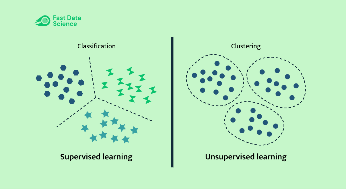
分類
監督式學習
supervised learning
機器學習
machine learning
非監督式學習
unsupervised learning
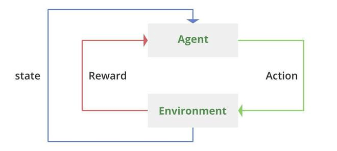
強化學習
reinforcement
learning
監督式學習
- 利用標籤數據(labeled data)學習
- 模型把自己的預測跟答案比較並精進
非監督式學習
- 利用無標籤數據(unlabeled data)學習
- 模型自己從資料中找到規律
強化學習
- AI跟"環境"作互動
- 得到獎勵或者懲罰
- 目標是得到最多的獎勵
- ex: 西洋棋電腦、機器人
A Starting Point
Decision Trees
Machine Learning
VS
Deep Learning
Machine Learning(機器學習)
Deep Learning
(深度學習)
決策樹

卷積神經網路
遞迴神經網路
圖神經網路

Deep Learning
- 神經網路
- 有很多"層"(可多達數百數千)
- 可以處理複雜的問題
- ex: ChatGPT (LLM)


- Pytorch
- Tensorflow
- Keras

Pytorch
Tensorflow
Keras


- Mid
- fast
- large data
- most used now
- hardest
- fast
- large data
- so called outdated
- Franchois Chollet
- easiest
- slower
- mid, little data
- good for learning
所以到底什麼是深度學習?
神經元
(neuron)
- 存數字
- 像一個格子
- 機率
Input Layer
...
Hidden Layers
Output Layer
簡化一下
0.3
0.7
0.1
0.9
0.4
0.3
0.3
資料

換成數字
換成其他形式
答案

影響
影響
如何影響?
0.7
0.3
這些連結會有所謂的權重(weight)
可以想像成不同神經連結有不同的強弱
0.4
0.4
1. 把每個神經元的值乘以連結的權重最後加起來
2. 加上偏差(bias)
0.2
3. 把數字帶入激勵函數
可減少線性度增加準確性
ex: sigmoid, softmax, ReLU...
0.8
-0.3
如何影響?
.
.
.
.
.
.
Yay! 你們已經理解了Forward Propogation
(前向傳播)
哪裡有學習?
偏差跟權重選什麼數字最好一開始都是隨機的,通過比較機器人預測的結果和標準答案,我們用某種演算法去一點一點修正我們的權重和數字,讓模型越來越好。
back propagation(反向傳播)
這東西小難,我們之後再講
back propagation(反向傳播)
MATH
統計的一些小東西
中位數(median)
眾數(mode)
平均值(mean)
平均值(mean)
標準差
(standard deviation)
變異數(variance)
線性回歸 linear regression
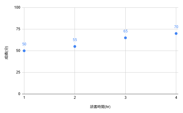
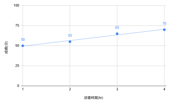
對我們要畫這條線
線性回歸 linear regression
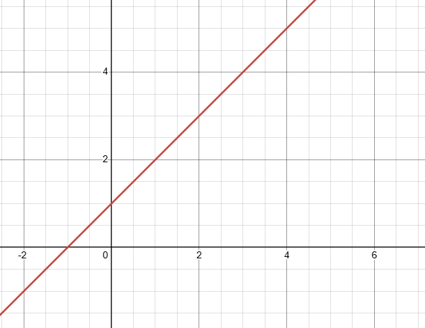
這是一條直線
這要用偏微分所以我就不證明了
但這是機器學習,所以我們要讓他自己學
何謂最好的直線?
誤差總和最小即是最好
其實這玩意已經有標準答案了
code
import matplotlib.pyplot as plt
import random


rng = random.SystemRandom()
x = [i for i in range(-50, 50, 1)]
y = [0.5 * i - 5 + rng.randint(-10, 10) for i in x]

a = rng.uniform(-1, 1)
b = rng.uniform(-1, 1)

print(f"intial linear equation: y = {a}x + {b}")

alpha_a = 0.0001
alpha_b = 0.01
epoch = 100

def line(x):
    return a*x + b

def delta_a(y, yh, x):
    return -2 * (y-yh) * x

def delta_b(y, yh):
    return -2 * (y-yh)

def correct_line():
    mean_x = sum(x) / 100
    mean_y = sum(y) / 100
    numerator = 0
    denominator = 0
    for i in range(100):
        numerator += (x[i] - mean_x) * (y[i] - mean_y)
        denominator += (x[i] - mean_x)**2

    correct_a = numerator / denominator
    correct_b = mean_y - correct_a*mean_x

    print(f"correct line: y = {correct_a}x + {correct_b}")


for _ in range(epoch):
    plt.clf()
    plt.plot([-50, 50], [0, 0], c = "black", alpha = 0.5)
    plt.plot([0, 0], [-50, 50], c = "black", alpha = 0.5)
    plt.xlim(-50, 50)
    plt.ylim(-50, 50)

    i = rng.randint(0, 99)
    yh = a*x[i] + b
    a -= alpha_a * delta_a(y[i], yh, x[i])
    b -= alpha_b * delta_b(y[i], yh)

    plt.plot([-50, 50], [line(-50), line(50)], c="red")
    plt.scatter(x, y, c="blue")
    plt.scatter(x[i], y[i], c="red")
    plt.pause(0.1)


print(f"final linear equation: y = {a}x + {b}")
correct_line()
code
import matplotlib.pyplot as plt
import random
用到的套件
matplotlib: 畫圖用
random: 隨機產生資料
pip install matplotlibrng = random.SystemRandom()
x = [i for i in range(-50, 50, 1)]
y = [0.5 * i - 5 + rng.randint(-10, 10) for i in x]
a = rng.uniform(-1, 1)
b = rng.uniform(-1, 1)隨機產生資料
隨機產生直線方程式的截距和斜率
print(f"intial linear equation: y = {a}x + {b}")

alpha_a = 0.0001
alpha_b = 0.01
epoch = 100
a跟b的調整單位
次數
code
def line(x):
    return a*x + b

def delta_a(y, yh, x):
    return -2 * (y-yh) * x

def delta_b(y, yh):
    return -2 * (y-yh)

def correct_line():
    mean_x = sum(x) / 100
    mean_y = sum(y) / 100
    numerator = 0
    denominator = 0
    for i in range(100):
        numerator += (x[i] - mean_x) * (y[i] - mean_y)
        denominator += (x[i] - mean_x)**2

    correct_a = numerator / denominator
    correct_b = mean_y - correct_a*mean_x

    print(f"correct line: y = {correct_a}x + {correct_b}")
迴傳模型生成的直線方程式的y值
每次如何調整a跟b
正確的線
梯度(gradient)函式:
用偏微分導出來的,我們之後會教這部分
code
for _ in range(epoch):
    plt.clf()
    plt.plot([-50, 50], [0, 0], c = "black", alpha = 0.5)
    plt.plot([0, 0], [-50, 50], c = "black", alpha = 0.5)
    plt.xlim(-50, 50)
    plt.ylim(-50, 50)

    i = rng.randint(0, 99)
    yh = a*x[i] + b
    a -= alpha_a * delta_a(y[i], yh, x[i])
    b -= alpha_b * delta_b(y[i], yh)

    plt.plot([-50, 50], [line(-50), line(50)], c="red")
    plt.scatter(x, y, c="blue")
    plt.scatter(x[i], y[i], c="red")
    plt.pause(0.1)
畫圖表
調整直線方程式
畫點跟線
print(f"final linear equation: y = {a}x + {b}")
correct_line()
下課!!!!!