Machine Learning
Full Course

講師 - 呂家睿
- 建中資訊38屆學術長+副社
- 玩雀魂
- 頭像是應急食品
- 被電爛
- 有問題歡迎來問我啊

- Fastapi
- Qt(C++)
- 數學好難
- 一點點sandbox
- Machine Learning
- discord bot
- 打開電腦
學術力

講師 - 林瑋浩
成功電研38屆教學
- 擅長寫O(2ⁿ)演算法
- 不會數學
- 回訊息很快
- C++
- Python
littleWeb前端- Discord bot
Bongosort- Machine Learning
- Godot
學術力

Review
Loss Function 損失函數
測量模型預測值與結果實際值差多少
MSE均方誤差
MAE平均絕對誤差
Cross Entropy交叉熵

Gradient Descent 梯度下降
讓誤差變小的方法
第n個世代
第n-1個世代
學習率
損失函數的梯度
Gradient Descent 梯度下降
讓誤差變小的方法
第n個世代
第n-1個世代
學習率
損失函數的梯度
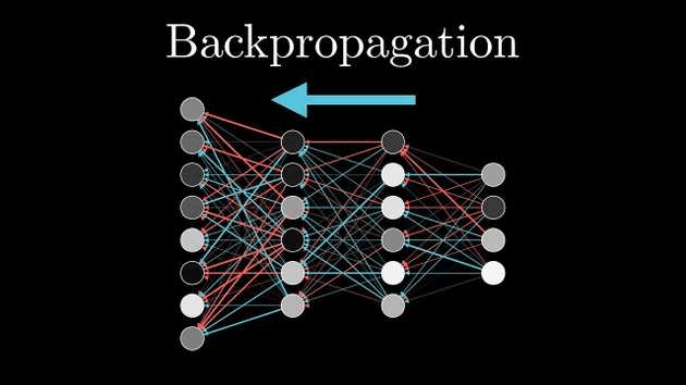
Backward Propagation
後向傳播
在模型預測完結果後,修正模型的過程
PyTorch
setup
venv 虛擬環境
一個獨立的環境,是一個大家很常用的好東西
- 乾淨、出問題好找
- 不會有太多套件混在一起
- 不同專案需要不同版本時不會衝突
1. 建立環境
python -m venv myenv2. 啟用環境
myenv\Scripts\activate //windows
source myenv/bin/activate //linux, mac
3. 安裝套件
pip install <package>pip-ing
使用這個套件要先把它下載好
pip install torch其他語言或套件請參考官網
CUDA
機器學習若欲使用GPU來加快運算,一個最常見的選項是nvidia的CUDA
可以在這裡下載
Tensor張量
Tensor張量
什麼是張量?
Scalar純量
vector向量
matrix矩陣
tensor張量
2D
1D
0D
- 基本上就是一個多維數組或者說多維陣列
- 深度學習的積木
Tensor張量
import torch
a = torch.tensor([[1,2],[2,3], [1,2]])
print(a)
b = torch.rand(2, 3, 4)
print(b)
c = torch.arange(0, 11, 5)
print(c)
d = torch.ones(2, 2)
print(d)
e = torch.zeros(3, 1)
print(e)
pytorch有專屬的tensor類別物件,有許多內建的強大功能
用現成資料創建一個tensor
創建指定大小,內容隨機的tensor - 建立新模型時會用到
- 類似for迴圈的方式
- 會回傳1D張量
創建內容全是一(或零)的tensor
Tensor張量
a = torch.rand(2, 2, dtype = None)
print(f"""
      Tensor a
      data type: {a.dtype}
      shape: {a.shape}
      device: {a.device}
      """)
b = torch.tensor([1,2], dtype = torch.int64)
print(f"""
      Tensor b
      data type: {b.dtype}
      shape: {b.shape}
      device: {b.device}
      """)

b = b.type(torch.float16)
print(b.dtype)
Tensor在pytorch中作為物件,有一些常用的物件屬性
dtype: tensor內資料的類別
shape: tensor的大小
device: tensor的位置
改變datatype
基本上deep learning 大部分的錯誤都跟這三個有關
Tensor張量
張量的四則運算,非常簡單,直接把對應的元素做加減乘除就好
a = torch.tensor([1, 2], [3, 4])
b = torch.tensor([5, 6], [7, 8])
print(a+b, torch.add(a, b))
print(a-b, torch.sub(a, b))
print(a*b, torch.mul(a, b))
print(a/b, torch.divide(a,b))
可以用直接打+-*/
或者是
用pytorch的函式
如果兩個張量沒辦法一一對應,缺的部分會自動補上
Tensor張量
希望你們還記得矩陣乘法
張量也有差不多的東西,在二維之上會比較複雜我們暫不討論
會加上batch跟broadcasting
1. 須滿足b = c
2. 乘出來的矩陣大小為a*d
Tensor張量
print(a@b, torch.matmul(a, b), torch.mm(a, b))任何狀況下都通用
只適用於矩陣(二維)的乘法,不能拿來用高維度的乘法
Tensor張量
print(a.mean())取得張量元素的平均值
如果tensor.dtype是整數類會報錯
print(a.argmax())
print(a.argmin())
會找到張量中最大和最小值得位置
ex:
a.argmax() = 3
a.argmin() = 0
Tensor張量
print(a.mean())取得張量元素的平均值
如果tensor.dtype是整數類會報錯
print(a.argmax())
print(a.argmin())
會找到張量中最大和最小值得位置
ex:
a.argmax() = 3
a.argmin() = 0
Tensor張量
tensor shape不符合怎麼辦?
a = torch.rand(3, 2, 1)

print(a.reshape(1, 2, 3))
b = a.view(1, 2, 3)
print(a, b)
b[0][0][0] = 1
print(a, b)
print(torch.stack([a, a, a ,a]))
reshape&view:
- 都能調整tensor的形狀
- 總元素數必須跟原來一樣多
- view創建出的物件記憶體和原物件是連通的
stack:
可以把tensor疊起來
Tensor張量
tensor shape不符合怎麼辦?
a = torch.rand(3, 2, 1)

print(a.reshape(1, 2, 3))
b = a.view(1, 2, 3)
print(a, b)
b[0][0][0] = 1
print(a, b)
print(torch.stack([a, a, a ,a]))
print(a.squeeze())
print(a.unsqueeze(dim = 0))
print(a.permute(2, 0, 1))
reshape&view:
- 都能調整tensor的形狀
- 總元素數必須跟原來一樣多
- view創建出的物件記憶體和原物件是連通的
stack:
可以把tensor疊起來
squeeze & unsqueeze:
可以幫tensor減一維或加一維
permute:
可以把維度互換
Auto Grad
Auto Grad
pytorch中最強的東西之一,可以把各個tensor"連在一起",並且自動幫你處理梯度
import torch
a = torch.rand(1, requires_grad = True)

b = a+3
c = b*3

print(f"""
      tensor a : {a}
      tensor b : {b}
      tensor c : {c}
      """)
看輸出之中會有一個grad_fn紀錄這個tensor最後做的運算
x3
+3

a
b
c
Auto Grad
用auto grad把所有tensor連起來之後,我們可以用 .backward()讓他自動計算梯度
c.backward()
print(a.grad)
a
b
c
x3
+3
一層一層回去計算梯度
把梯度存在a.grad
Auto Grad
以最簡單的例子而言,我們現在長這樣:
根據梯度調整w, b
輸入
輸出
.backward()取得梯度
計算誤差
Initialize 初始化
import torch

w = torch.rand(1, requires_grad = True)
b = torch.rand(1, requires_grad = True)

epochs = 100
learning_rate = 0.1

print(f"""
      Initial values:
      w = {w}
      b = {b}\n
      """)
隨機取數weight和bias
epoch 訓練週期
learning rate 一次要調多少
Code

Code
for epoch in range(epochs):
    x = torch.rand(1)
    y = 2*x + 1
    y_hat = w*x + b
    loss = (y_hat - y)**2


    loss.backward()

    with torch.no_grad():
        w -= learning_rate*w.grad
        b -= learning_rate*b.grad

        w.grad.zero_()
        b.grad.zero_()

    if epoch % 10 == 0:
        print(f"""
              At epoch {epoch}:
              w = {w}
              b = {b}\n
              """)
print(f"""
        Final value:
        w = {w}
        b = {b}\n
        """)
計算誤差值
back prop
training 訓練
把梯度歸零
不追蹤grad_fn
pytorch.nn
pytorch.nn
所以我們之前要手動操作各個weight跟bias很麻煩
可以使用pytorch內建的工具來幫我們處理神經網絡
model = nn.Linear(in_features = 1, out_features = 1)

epoch = 100
learning_rate = 0.1

critereon = nn.MSELoss()

print(f"""
      Initial values:
      w = {model.weight}
      b = {model.bias}\n
      """)
創建一個nn.Linear物件
損失函數的計算函式
Initialize 初始化
pytorch.nn
for epoch in range(epochs):
    x = torch.rand(1)
    y = 2*x + 1
    y_hat = model(x)
    loss = critereon(y_hat, y)

    loss.backward()

    with torch.no_grad():
        for param in model.parameters():
            param -= learning_rate *param.grad


    model.zero_grad()

    if epoch % 10 == 0:
        print(f"""
              At epoch {epoch}:
              w = {model.weight}
              b = {model.bias}\n
              """)
print(f"""
        Final value:
        w = {model.weight}
        b = {model.bias}\n
        """)
training 訊練
預測
計算誤差
更新
for epoch in range(epochs):
    x = torch.rand(1)
    y = 2*x + 1
    y_hat = model(x)
    loss = critereon(y_hat, y)

    loss.backward()

    with torch.no_grad():
        for param in model.parameters():
            param -= learning_rate *param.grad


    model.zero_grad()

    if epoch % 10 == 0:
        print(f"""
              At epoch {epoch}:
              w = {model.weight}
              b = {model.bias}\n
              """)
print(f"""
        Final value:
        w = {model.weight}
        b = {model.bias}\n
        """)
重設梯度
稍微難一點的code
import torch
import torch.nn as nn
import math
import matplotlib.pyplot as plt


x = torch.linspace(-math.pi, math.pi, 1000).unsqueeze(1)
y = torch.sin(x)

model = nn.Sequential(
    nn.Linear(1, 32),
    nn.Tanh(),
    nn.Linear(32, 32),
    nn.Tanh(),
    nn.Linear(32, 1)
)

criterion = nn.MSELoss()

learning_rate = 0.01
epochs = 5000
準備資料
建立模型
Intialize 初始化
稍微難一點的code
for epoch in range(epochs):
    y_hat = model(x)

    loss = criterion(y_hat, y)
    loss.backward()

    with torch.no_grad():
        for param in model.parameters():
            param -= learning_rate * param.grad

    model.zero_grad()

    if epoch % 500 == 0:
        print(f"Epoch {epoch:4} | Loss: {loss.item():.4f}")

print("Training complete!")
基本上跟之一樣
Training 訓練
稍微難一點的code
predictions = model(x).detach()

plt.figure(figsize=(8, 4))
plt.plot(x.numpy(), y.numpy(), label="True Sine Wave", color="blue", linewidth=2)
plt.plot(x.numpy(), predictions.numpy(), label="Prediction", color="red", linestyle="dashed", linewidth=2)
plt.legend()
plt.title("Predict Sine Wave")
plt.show()
這裡用的是matplotlib
畫圖呈現
畫一條藍色的代表真正的sin函數
紅色代表預測的值
練習題
訓練一個模型讓他預測
import torch
import torch.nn as nn
import matplotlib.pyplot as plt

x = torch.linspace(-5, 5, 1000).unsqueeze(1)
y = x**3 + 2*x + 1


model = nn.Sequential(
    nn.Linear(1, 32),
    nn.Tanh(),
    nn.Linear(32, 32),
    nn.Tanh(),
    nn.Linear(32, 1)
)

criterion = nn.MSELoss()
learning_rate = 0.01

epochs = 2000
for epoch in range(epochs):
    y_hat = model(x)

    loss = criterion(y_hat, y)
    loss.backward()
    with torch.no_grad():
        for param in model.parameters():
            param -= learning_rate * param.grad

    model.zero_grad()

    if epoch % 500 == 0:
        print(f"Epoch {epoch:4} | Loss: {loss.item():.4f}")

print("Training Complete!")


predictions_plot = model(x).detach()

plt.figure(figsize=(8, 5))
plt.plot(x.numpy(), y.numpy(), label="True Curve (y = x^3 + 2x + 1)", color="blue", linewidth=2)
plt.plot(x.numpy(), predictions_plot.numpy(), label="Prediction", color="red", linestyle="dashed", linewidth=2)
plt.legend()
plt.title("Predicting Cubic")
plt.xlabel("x")
plt.ylabel("y")
plt.show()
下課!!!!!