Total Functions for Automated Reasoning
Building Terminating Theorem Provers
Alexander Gryzlov
(IMDEA Software Institute)
Lambda World 2025
October 24, Cádiz, Spain

Agenda
- AI & automated reasoning
- Total programming
- Unification
- SAT & DPLL
- Iterative DPLL
As you can guess/deduce from the title, this is a talk about combining two topics I've been working on for the past couple of years.
Agenda
- AI & automated reasoning
- Total programming
- Unification
- SAT & DPLL
- Iterative DPLL
Part 1
The domain:
AI & Automated Reasoning
AI is somewhat like "teenage music".
For every decade, it could mean something different:
- 1960s - The Beatles & Expert systems
- 1990s - Backstreet Boys & Spam filter/recommenders
- 2020s - Ariana Grande & Large Language Models
Let us go back to the basics!
AI through time


Classic AI tasks
- Machine translation and text comprehension
- Speech and pattern recognition
- Game playing (chess, checkers, Go, etc)
- Theorem proving
Formulated back in 1950s as "human-level activities performed by computer:"
We'll focus on the last one:
Here, symbolic (rather than statistical) methods are typically used, and precise guarantees matter the most.
Theorem proving landscape
- SAT/SMT solvers (Z3/cvc5)
- Computer algebra systems (Mathematica, MAPLE)
- Automated provers (Vampire, E, iProver)
- Logic programming languages (Prolog, λProlog, Datalog)
- Proof assistants (HOL, Coq, Agda, Lean)
There's a struggle between the power of the system and automation.
More versatile systems converge toward general-purpose programming languages.
Automation vs power
We'll use an interactive tool (Agda) to build and verify some simple automated ones.
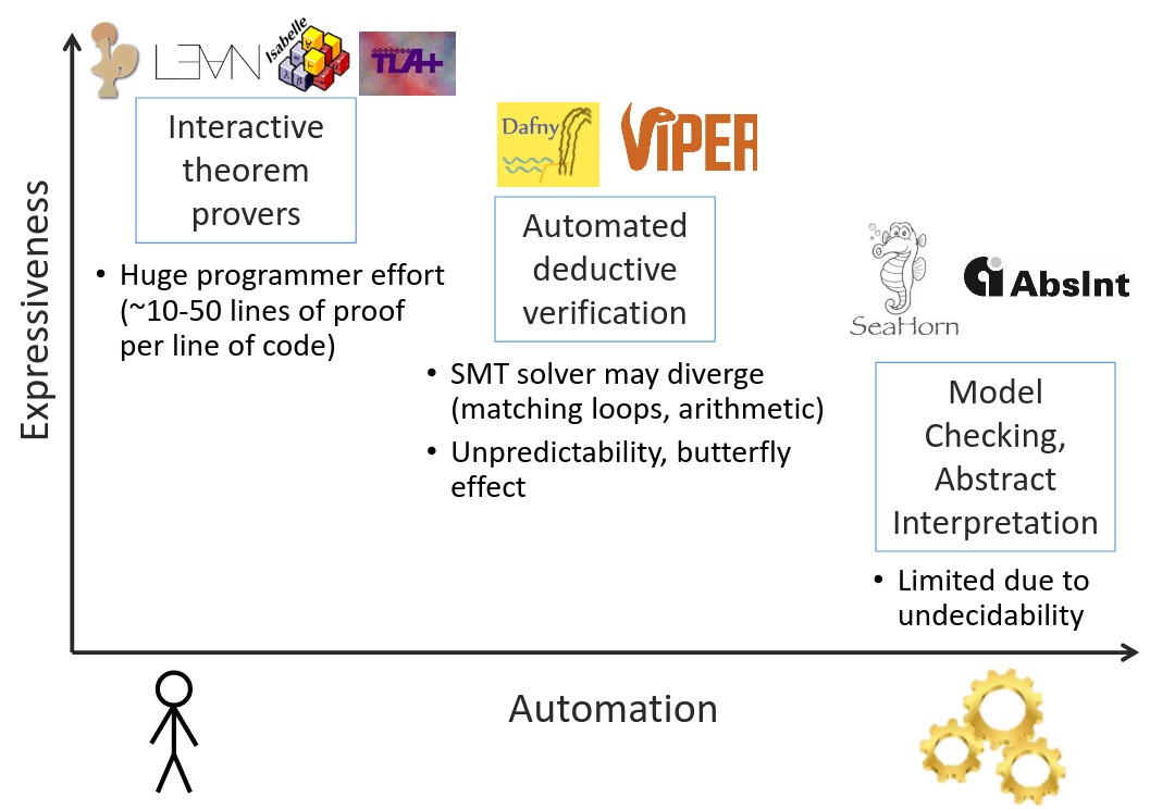
Shoham, [2019] "Verification of Distributed Protocols Using Decidable Logic"
Automated reasoning
The subfield of symbolic AI focused on theorem proving is referred to as "automated reasoning."
Typically involves:
- operating on syntax with variables
- synthesizing terms/proofs/refutations (not always)
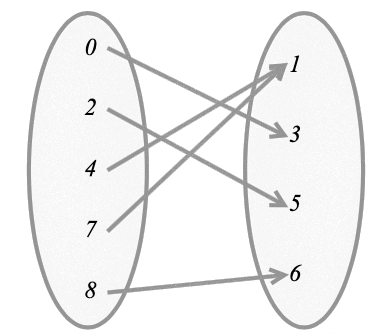
- computing finite representations of functions (maps)
The algorithms we'll see use first-order syntax:
no binders (like λ) inside terms.
Variables and contexts
An important notion when reasoning about variables: context.
This is what logicians/type theorists write as capital Greek letters (Γ/Δ).
A finite set of all variables in the expression.
An overapproximation - can include extra variables not in the term!
We'll use a special (quotient) type Ctx for sets of variables (the order and multiplicity in it don't matter).
Has the usual set operators and predicates: ∈, union, rem, minus
Part 2
The technique:
Total programming
The nature of functions
We're going to compute maps/functions, but can we be precise about them?
(Pure) functions in FP are close to the mathematical definition of a function.
But how do we guarantee the "each" and "exactly one" part?
a function from a set X to a set Y assigns to each element of X exactly one element of Y
Computational functions
Two problems beyond purity:
- not every X is assigned a Y
- a Y is never produced
head :: [a] -> a
head []    = error "oops"
head (x:_) = x
loop :: a -> a
loop x = loop xTermination matters
Can be costly in critical systems, we typically expect each request/component to finish, even if the system is interactive:
916 such CVE’s between 2000 and 2022
"Large-scale analysis of non-termination bugs in real-world OSS projects" (2022)
For reasoning algorithms, this means we always get an answer (though it may take a long time).
Total programming
We can only write programs which:
- cover all inputs
- terminate
The first part is relatively trivial (though often requires restructuring your program),
however the second involves recursion :(
Structural recursion
Programs which "consume" syntactically smaller pieces of input:
data Tree : 𝒰 where
  leaf : Tree
  node : Tree → Tree → Tree

depth : Tree → ℕ
depth leaf         = 0
depth (node l r)   = 1 + max (depth l) (depth r)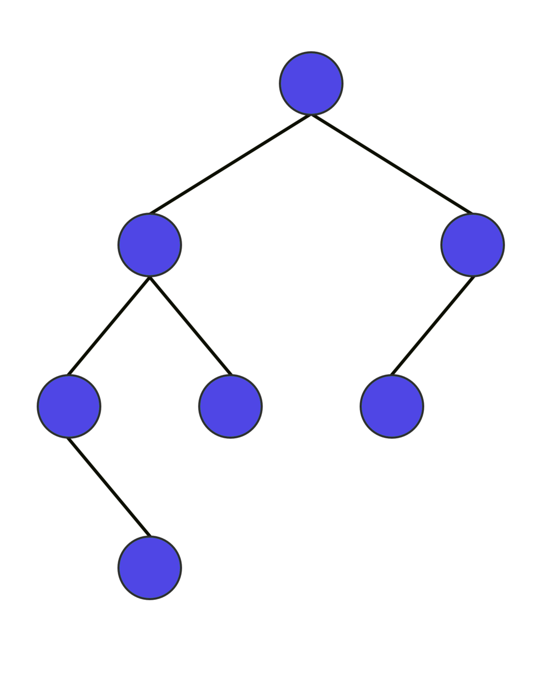
Beyond structural
Here's a simple example that doesn't fit this pattern:
Euclid's GCD algorithm
{-# TERMINATING #-}
gcd : ℕ → ℕ → ℕ
gcd n m =
  if m == 0
    then n
    else gcd m (n % m)
We know n % m < m but this is not structural!
gcd(105, 30) → 105%30 = 15
gcd(30, 15) → 30%15 = 0
gcd(15, 0) = 15
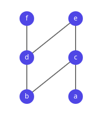
Well-founded recursion
We have to introduce a "measure" that decreases on a type T according to a well-founded order.
If you come up with any sequence ... < tx < ty < tz < ..., it cannot decrease forever.
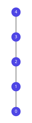
A canonical type with such an order is (ℕ, <).
Any sequence will eventually end with 0.
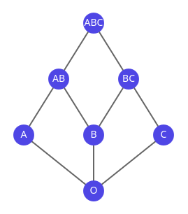
Called a linear order, but orders can be branching.
Well-founded language
Let's introduce a special type for this goal:
record □_ (A : T → 𝒰) (x : T) : 𝒰 where
  field call : (x : T) → y < x → A y

-----------------

fix : (A : T → 𝒰)
    → ({t : T} → □ A t → A t)
    → ({t : T} → A t)

-- a non-total fixpoint would be
-- fix : (A → A) → A
□A means "A can only be called with an argument smaller than its index".
If the order is well-founded, we can implement the fixed-point combinator!
Well-founded language - sugar
-- implicit
fix : (A : T → 𝒰)
   → ({t : T} → □ A t → A t)
   → ({t : T} → A t)

-- sugar!
fix : (A : T → 𝒰)
   → ∀[ □ A ⇒ A ]
   → ∀[ A ]
Sometimes we want to hide the decreasing argument (make it implicit), other
times it's crucial to computation.
-- explicit
fix : (A : T → 𝒰)
   → ((t : T) → □ A t → A t)
   → ((t : T) → A t)

-- sugar!
fix : (A : T → 𝒰)
   → Π[ □ A ⇒ A ]
   → Π[ A ]
Well-founded GCD
Here's an example of computing a GCD function like this (uses the explicit form):
gcd-ty : ℕ → 𝒰
gcd-ty x = (y : ℕ) → y < x → ℕ

gcd-loop : Π[ □ gcd-ty ⇒ gcd-ty ]
gcd-loop x rec y y<x =
  caseᵈ y = 0 of
    λ where
        (yes y=0) → x
        (no y≠0) →
          rec .call
  -- it is safe to do the recursive call
            y<x (x % y)
  -- remainder is smaller
            (%-r-< x y
              (≱→< $ contra ≤0→=0 y≠0))
gcd< : Π[ gcd-ty ]
gcd< = fix gcd-ty gcd-loop
gcd : ℕ → ℕ → ℕ
gcd x y =
caseᵗ x >=< y of
λ where
(LT x<y) → gcd< y x x<y
(EQ x=y) → x
(GT y<x) → gcd< x y y<xTo kick-start the computation, we just need to decide which argument goes first:
Part 3
The tutorial level:
Unification
Sometimes called "a Swiss army knife operator".
A family of (semi)algorithms for solving equations.
Match a pattern with gaps in it against data to fill the gaps.
Many applications:
- logic programming
- type inference
- 1st order logic provers
- program synthesis
- ...
Unification

Most General Unifier
First-order MGU: a classical form described in Pierce's TAPL.
Given a pair of terms (or generally a list of pairs),
find a substitution that makes all of them equal (or fail):
A     ≟ A      {}
A     ≟ B        FAIL
A     ≟ x      { x ↦ A }
A     ≟ B ⊗ C    FAIL
x     ≟ B ⊗ C  { x ↦ B ⊗ C }
x ⊗ B ≟ A ⊗ y  { x ↦ A , y ↦ B }
x     ≟ x ⊗ x    FAIL
[ x   ≟ y
, y   ≟ A ]    { x ↦ A , y ↦ A }
Terms & constraints
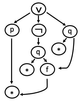
data Term : 𝒰 where
  ``_ : Var → Term
  _⊗_ : Term → Term → Term
  sy  : String → Term

-- x ⊗ B
example : Term
example = `` x ⊗ sy "B"

Constr : 𝒰
Constr = Term × Term- Terms are just binary trees with two kinds of leaves
- Variables are an abstract type with equality (think ℕ/String)
- Constraints are pairs of terms
We need both internal and external substitution:
-- internal
sub1 : Var → Term → Term → Term
sub1 v t (`` x)  =
  if v == x then t else `` x
sub1 v t (p ⊗ q) =
  sub1 v t p ⊗ sub1 v t q
sub1 v t (sy s) =
  sy s

subs1 : Var → Term → List Constr → List Constr

-- external
Sub : 𝒰
Sub = Map Var Term
Unification code
unify : List Constr → Maybe Subst
unify []              = just emptyM
unify ((tl, tr) ∷ cs) =
  if tl == tr
     then unify cs
     else unifyHead tl tr cs

unifyHead : Term → Term
          → List Constr → Maybe Subst
unifyHead (`` v)      tr        cs =
  if occurs v tr then nothing
    else map (insertM v tr) $
         unify (subs1 v tr cs)
unifyHead  tl         (`` v)    cs =
  ... -- symmetrical
unifyHead (lx ⊗ ly) (rx ⊗ ry) cs =
  unify ((lx , rx) ∷ (ly , ry) ∷ cs)     -- adds constraints!
unifyHead _          _          _  =
  nothing
Why does it terminate?
- Can't just count constraints - they increase for the ⊗ case
- Option 1: context size (count variables) - substitution removes variables; however, the context size stays the same for ⊗
- Option 2: count total term size in constraints - decreases for ⊗ (one level gets dismantled), but can grow for var case
tm-size : Term → ℕ
tm-size (p ⊗ q) = 1 + tm-size p + tm-size q
tm-size _       = 1

tm-sizes : List Constr → ℕ
Solution: combine 1 and 2!
Lexicographic order
We can combine two (or generally N) well-founded orders:
(a,b) < (x,y) := a < x OR (a = x AND b < y)
One component always decreases!
For unification this means:
- Either context decreases (var case),
- Or it stays the same but the total term size does (⊗ case)
Input : 𝒰
Input = Ctx × List Constr

wf-tm : Ctx → Term → 𝒰
wf-tm c t = vars t ⊆ c

wf-input : Input → 𝒰
-- each term in the constraint
-- list is WF
unify-ty : ℕ × ℕ → 𝒰
unify-ty (x , y) =
(inp : Input)
→ wf-input inp
→ x = size (inp .fst)
→ y = term-sizes (inp .snd)
→ Maybe Sub
Terminating case for ⊗
-- before
unifyHead (lx ⊗ ly) (rx ⊗ ry) cs =
  unify ((lx , rx) ∷ (ly , ry) ∷ cs)

-- after
unify-head-loop rec (ctx , cs) wf (lx ⊗ ly) (rx ⊗ ry) wl wr ex ey =
  rec .call prf-<
     (ctx , ls') prf-wf
     refl refl
  where
  cs' : List Constr
  cs' = (lx , rx) ∷ (ly , ry) ∷ cs
  prf-< : (size ctx , term-sizes cs') < (size ctx , term-sizes cs)
  prf-< = ...
  prf-wf : wf-input (ctx , cs')
  prf-wf = ...
Part 4
The main quest:
SAT & DPLL
The SAT problem
Classical constraint satisfaction task:
Given a boolean formula with variables,
find an assignment of variables that makes it true (or fail).
Compared to unification:
- we restrict the range of variables (only True/False)
- but we add a semantical constraint (Boolean evaluation)
The SAT problem examples
-- tautologies (true for every assignment)

True
P ∧ Q ⇒ P ∨ Q
((P ⇒ Q) ⇒ P) ⇒ P  -- aka Peirce's law

-- satisfiable (there is an assignment)

P ∧ Q ⇒ Q ∧ R        -- P = Q = True, R = False
                      -- simplifes to True ⇒ False

-- unsatisfiable

P ∧ ¬P
Exponential search
- The most widely used approach is backtracking search
- Naively we can try each variable and flip a previous choice when getting
False - However that's 2ⁿ operations where n = #variables
- Can we do better?
Generally, in the worst case, no! :(
Cook–Levin theorem (1971): SAT is NP-complete
(btw, this is the birth of NP-completeness concept).
But some heuristics can make less-than-worst cases tractable.
DPLL
Davis–Putnam–Logemann–Loveland algorithm, 1961
- Still fundamentally performs backtracking search
- But uses 3 heuristics to prune the search substantially
- These are unit propagation, pure literal rule and literal selection
CNF
DPLL and similar algorithms assume the input is in a
conjunctive normal form: a big conjunction of disjunctions of possibly negated literals (clauses)
  ( A ∨ ¬B)
∧ (¬C ∨  D ∨ E)
∧ ...
We can always transform into one thanks to boolean reasoning principles (i.e. DeMorgan rule: ¬(P ∨ Q) = ¬P ∧ ¬Q)
True            ~  ∅
False           ~  ()
P ∨ Q           ~  (P ∨ Q)
P ∧ Q           ~  (P) ∧ (Q)
P ∧ Q ⇒ Q ∧ R   ~  (¬P ∨ ¬Q ∨ R)
CNF encoding
data Lit (Γ : Ctx) : 𝒰 where
  Pos : (v : Var) → v ∈ Γ → Lit Γ
  Neg : (v : Var) → v ∈ Γ → Lit Γ

var : Lit Γ → Var
var (Pos v _) = v
var (Neg v _) = v

positive : Lit Γ → Bool
positive (Pos _ _) = true
positive  _        = false
Unlike in unification, we push the well-formedness constraint into the literals:
Clause : Ctx → 𝒰
Clause Γ = List (Lit Γ)

CNF : Ctx → 𝒰
CNF Γ = List (Clause Γ)

literals : CNF Γ → List (Lit Γ)
literals = nub ∘ concat
Unit propagation aka 1-literal rule
unit-clause : CNF Γ → Maybe (Lit Γ)
unit-clause  []               = nothing
unit-clause (        []  ∷ c) = unit-clause c
unit-clause ((x ∷    []) ∷ c) = just x
unit-clause ((_ ∷ _ ∷ _) ∷ c) = unit-clause c

unit-propagate : (l : Lit Γ) → CNF Γ → CNF (rem (var l) Γ)
unit-propagate l []      = []
unit-propagate l (f ∷ c) =
  if has l f
    then unit-propagate l c
    else delete-var (var l) f ∷ unit-propagate l c

one-lit-rule : CNF Γ → Maybe (Σ[ l ꞉ Lit Γ ] (CNF (rem (var l) Γ)))
one-lit-rule cnf =
  map (λ l → l , unit-propagate l cnf) $
  unit-clause cnf
Heuristic 1: If a clause consists of a single literal, it must be true, propagate it through the formula:
  (A ∨ ¬B)
∧ (C)
∧ ...
Pure literal rule
pure-literal-rule :
    (c : CNF Γ)
  → (Σ[ purelits ꞉ List (Lit Γ) ]
      (let vs = map var purelits in
      (vs ≬ Γ) × CNF (minus Γ vs)))
  ⊎ (∀ {l} → l ∈ literals c → negate l ∈ literals c)
...
Heuristic 2 (aka affirmative-negative rule):
The idea is to delete every literal that occurs strictly positively or strictly negatively (purely).
Literal selection
posneg-count : CNF Γ → Lit Γ → ℕ
posneg-count cnf l =
  let m = count (has          l) cnf
      n = count (has $ negate l) cnf
    in
  m + n

splitting-rule : (c : CNF Γ)
               → Any positive (literals c)
               → Lit Γ
The previous two rules try to eliminate guessing as much as possible, but eventually, we're going to have to guess a value.
This is where backtracking still happens.
The splitting rule guarantees a result after the pure literal one.
Putting it all together
Answer = Map Var Bool

dpll-loop : (CNF Γ → Maybe Answer)
           → CNF Γ → Maybe Answer
dpll-loop rec cnf =
  if null? cnf then just emptyM       -- trivially true
    else if has [] cnf then nothing   -- trivially false
      else
        maybe
          (maybe
             (let l = splitting-rule cls in
              map (either (insertLit l)
                          (insertLit (negate l))) $
                  rec (unit-propagate l cnf)
              <+> rec (unit-propagate (negate l) cnf))
             (λ (ls , c) → map (insertLits ls) $ rec c)
             (pure-literal-rule cnf))
          (λ (l , c) → map (insertLit l) $ rec c)
          (one-lit-rule cnf)
Why does this terminate?
Context always decreases:
- For unit propagation by 1
- For pure literal by some n ≥ 1
- For recursive call by 1
This is actually simpler than unification!
We don't need the lexicographic pair, just a single number:
DPLL-ty : ℕ → 𝒰
DPLL-ty x =
    {Γ : Ctx}
  → x = size Γ
  → CNF Γ → Maybe Answer
Part 5
The boss fight:
Iterative DPLL
Iterative DPLL
- Again, the core of the algorithm is backtracking search
- However, the backtracking information is kept on the system stack - no tail recursion
- Actual implementations work tail-recursively (iteratively)
...
  (map (either (insertLit l)
               (insertLit (negate l))) $
       rec (unit-propagate l cls)
   <+> rec (unit-propagate (negate l) cls))
...
Trail blazing
- We make the stack a first-class object, usually called a trail
- Need add a flag do determine if the literal is guessed, which then serves as a backtrack point
data Flag : 𝒰 where
  guessed deduced : Flag

Trail : Ctx → 𝒰
Trail Γ = List (Lit Γ × Flag)

trail-lits : Trail Γ → List (Lit Γ)
trail-lits = map fst

trail→answer : Trail Γ → Answer
trail→answer =
  fold-r emp λ (l , _) → upd (var l) (positive l)
Heuristics redux
unit-subpropagate-loop : (CNF Γ → Trail Γ → CNF Γ × Trail Γ)
                       →  CNF Γ → Trail Γ → CNF Γ × Trail Γ
unit-subpropagate-loop rec cnf tr =
  let cnf' = map (filter (not ∘ trail-has tr ∘ negate)) cnf
      newunits = literals (filter (is-fresh-unit-clause tr) cnf')
    in
  if null newunits
    then (cnf' , tr)
    else loop cnf' (map (λ l → l , deduced) newunits ++ tr)
We get rid of the pure literal rule but perform unit propagation in batches:
Iterative DPLL loop
backtrack : Trail Γ → Maybe (Lit Γ × Trail Γ)
backtrack []                   = nothing
backtrack ((_ , deduced) ∷ ts) = backtrack ts
backtrack ((p , guessed) ∷ ts) = just (p , ts)

dpli-loop : CNF Γ
         → (Trail Γ → Maybe Answer)
         →  Trail Γ → Maybe Answer
dpli-loop cnf rec tr =
  let (cnf' , tr') = unit-subpropagate cnf tr in
  if has [] cnf' then          -- reached False
      maybe
        nothing
        (λ (p , trb) → rec ((negate p , deduced) ∷ trb))
        (backtrack tr)
    else
      ...
Then we either run into an inconsistency and have to backtrack:
Iterative DPLL loop
dpli-loop : CNF Γ
         → (Trail Γ → Maybe Answer)
         →  Trail Γ → Maybe Answer
dpli-loop cnf rec tr =
  let (cnf' , tr') = unit-subpropagate cnf tr in
  if has [] cnf' then
      ...
    else               -- need to guess
      let ps = unassigned cls tr' in
      if null ps
        then just (trail→answer tr')
        else rec ((splitting-rule' cls ps , guessed) ∷ tr)
Or we have to make a choice:
Why does any of this terminate?
For unit propagation, the measure is the count of literals still unused in the trail:
(x2 because of polarity)
y = 2 · size Γ ∸ length trHowever this, only works when the trail is unique (invariant #1)
Main loop termination
For the guess case, the unused trail literals also work:
We take the old trail and add a new literal onto it, exhausting unused ones.
But what about the backtracking case?
Here trb is a suffix of the old trail - it shrinks!
We had the same situation in unification: two kinds of recursive calls, one decreases a measure, the other one increases.
Looks like we need to use the lexicographic product again, but with what?
rec ((splitting-rule' cls ps , guessed) ∷ tr)rec ((negate p , deduced) ∷ trb)Main loop termination - idea
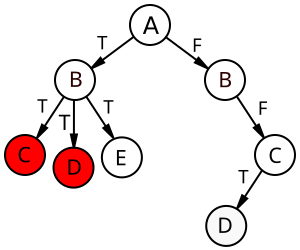
- Intuitively, it's the search space that decreases for backtracking
- But the search tree is generated on the fly
- We need to find a proxy
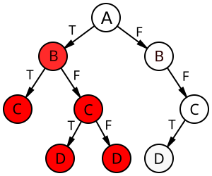
If we look closely at this tree, we notice that
we never return to discarded branches.
So what sticks around is rejected literals.
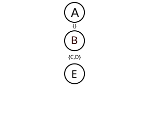
Main loop termination - measure
- However, we can't lump them all together - the deduced literals get discarded after backtracking.
- We need to keep a vector of these rejected sets.
- The first part of the measure, then, is a vector of counts of still-available literals.
The full measure is then a lexicographic product of a vector (N-ary product) of non-rejected assignments corresponding to the guessed level and the number of unused variables in the trace!
(whew)
DPLI termination invariants
For all of this to work, we need the old trail uniqueness invariant and a new one:
- Variable + polarity should not repeat
- If a guessed variable is in the trail, its negation doesn't appear before it
The rejected vector/stack also needs an invariant:
If a variable is on level n, its negation appears in the trail after dropping the first n guessed variables.
Just need to prove that all of these are preserved :/
Uniq (trail-lits tr) ×
  (∀ x → (x , guessed) ∈ tr
       → negate x ∉ tail-of x (trail-lits tr))

∀ x (f : Fin (size Γ))
   → x ∈ lookup rj f
   → negate x ∈ (trail-lits $ drop-guessed tr (count-guessed tr ∸ fin→ℕ f))
DPLI termination type
DPLI-ty : {Γ : Ctx} → Vec ℕ (size Γ) × ℕ → 𝒰
DPLI-ty {Γ} (x , y) =
    (tr : Trail Γ)
  → Trail-invariant tr
  → (rj : Rejectstack Γ)
  → Rejectstack-invariant rj tr
  → x = map (λ q → 2 · size Γ ∸ size q) rj
  → y = 2 · size Γ ∸ length tr
  → Maybe Answer
Conclusion
Lessons learned
- Writing out termination proofs forces you to understand how the algorithm actually works, in the form of its invariants.
- Control flow tricks make termination harder :(
- Once you determine the invariants, you have more freedom to restructure your algorithm, make it more modular, experiment with different representations, and so on.
Lessons learned
- More generally, from a mathematical point of view, automated reasoning is about syntax, finite sets, maps, and intricate order relations.
- And order theory is just a cut-down version of category theory, but that is a story for another time...
References
- Automated Reasoning @ SEP
- Shi, Xie, Li, Zhang, Chen, Li, [2022] "Large-scale analysis of non-termination bugs in real-world OSS projects"
-
Cook, Podelski, Rybalchenko, [2011] "Proving program termination"
-
Hoder, Voronkov, [2009] "Comparing unification algorithms in first-order theorem proving"
-
Vardi, [2015] "The SAT Revolution: Solving, Sampling, and Counting"
-
Harrison, [2009] "Handbook of Practical Logic and Automated Reasoning"
Contacts & repo


Acknowledgments
Partially funded by the European Union (GA 101039196). Views and opinions expressed are however those of the author(s) only and do not necessarily reflect those of the European Union or the European Research Council. Neither the European Union nor the European Research Council can be held responsible for them.