Intro to Causal Inference and Regression
About
- Understand causal inference
- How we can use regression in causal inference
- Examples!

About
- Understand causal inference
- How we can use regression in causal inference
- Examples!
Myself
- Cam Davidson-Pilon
- Former Director of Data Science at Shopify
- Author of popular Python libraries, lifelines and Bayesian Methods for Hackers
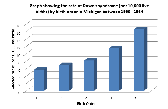
Does birth order cause Down's Syndrome?
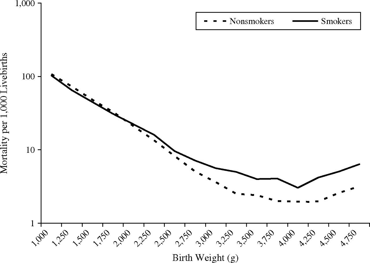
Does smoking reduce infant mortality?
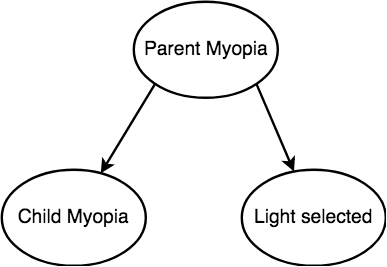
Do nightlights cause myopia?
Does being good at programming contests negatively impact work performance?
Causal Diagrams
Causal Directed Acycle Graphs represent our apriori, domain knowledge about the relationship between variables.
Vertices are variables, and a directed edge's tail is the cause of the directed edge's head.
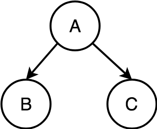
A causes B, and A causes C. (A is a confounder)
1. B and C are independent, conditioned on A.
2. B and C are correlated, unconditioned on A.
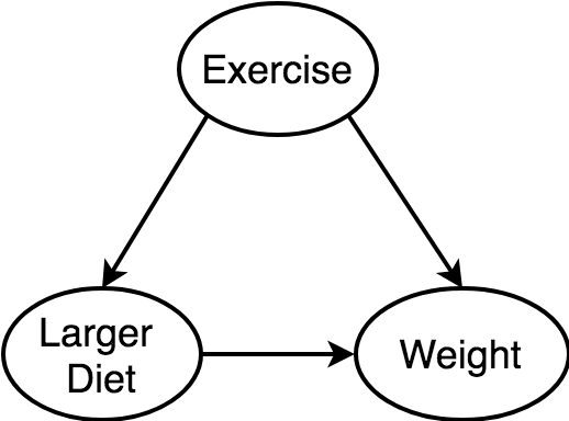
Example: merchant sales causes both retention and higher plans
Common Cause (Confounders)
Ignoring the common cause (maternal age) of birth order and incidence of Down's syndrome, introduces a spurious relationship between the child nodes.
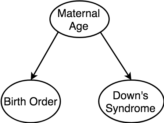
Common Cause (Confounders)
Common Effect (Colliders)
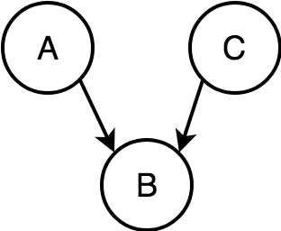
A causes B, and C causes B.
1. A and C are independent, unconditioned on B.
2. A and C are correlated, conditioned on B.
Common Effect (Colliders)
| A | B | C |
|---|---|---|
| 0 | 1 | 1 |
| 1 | 0 | 1 |
| 1 | 1 | 1 |
| 0 | 0 | 0 |
No conditioning on C
| A | B | C |
|---|---|---|
| 0 | 1 | 1 |
| 1 | 0 | 1 |
| 1 | 1 | 1 |
| 0 | 0 | 0 |
Conditioning on C = 1
Common Effect (Colliders)
| A | B | C |
|---|---|---|
| 0 | 1 | 1 |
| 1 | 0 | 1 |
| 1 | 1 | 1 |
| 0 | 0 | 0 |
No conditioning on C
| A | B | C |
|---|---|---|
| 0 | 1 | 1 |
| 1 | 0 | 1 |
| 1 | 1 | 1 |
| 0 | 0 | 0 |
Conditioning on C = 1
What is the correlation between A & B in these two tables?
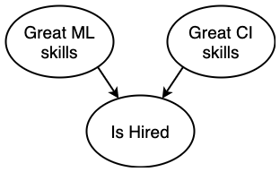
Both great ML skills and great CI skills can get a data scientist hired, so
There is a negative correlation between great ML skills and great CI skills, given the data scientist is hired at a company.
Common Effect (Colliders)
Common Effect (Colliders)
Common Effect (Colliders)

Chains
A causes B, and B causes C.
1. A and C are independent, conditioned on B.
2. A and C are correlated, unconditioned on B.
Example: Attending high school causes Attending university causes Attending grad school

Larger DAGs
We can of course have large DAGs, and the same biases hold:
1. Conditioning on common effects introduces a bias
2. Not conditioning on common causes introduces a bias
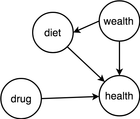
So how do we now what to condition for?
1. Ask a precise question
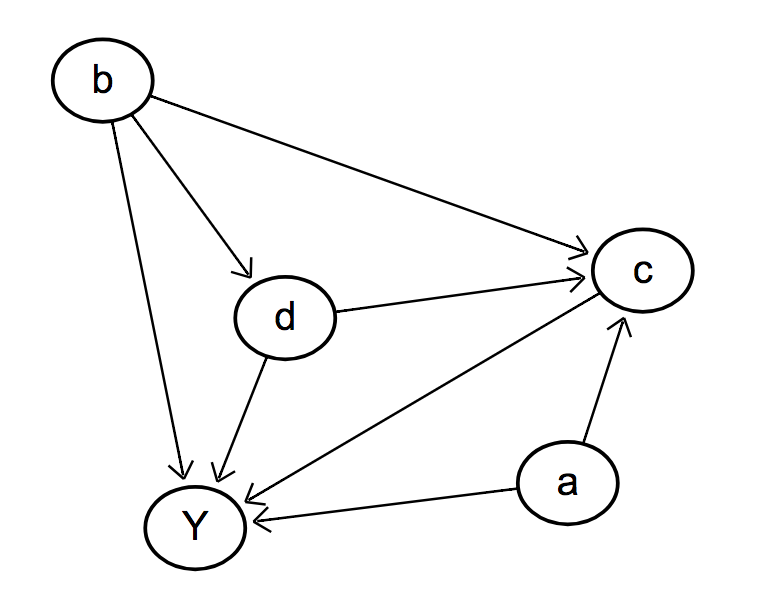
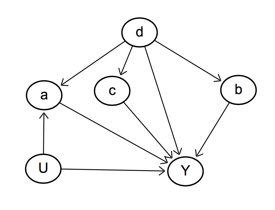
We need to ask a more precise question. Let's focus on the diagram to the right and ask:
"What is the total effect of d on Y?"
1. Ask a precise question
We need to ask a more precise question. Let's focus on the diagram to the right and ask:
"What is the total effect of d on Y?"
1. Ask a precise question
We need to ask a more precise question. Let's focus on the diagram to the right and ask:
"What is the total effect of d on Y?"
1. Ask a precise question
We need to ask a more precise question. Let's focus on the diagram to the right and ask:
"What is the total effect of d on Y?"
We can apply the backdoor criteria to know what to control for.
2. Backdoor criteria
Find a set of nodes, Z, s.t.
1. No node in Z is a descendant of d.
2. Z blocks every path between d and Y that contains an arrow into d.
The first condition handles common effects, the second condition handles common causes.
2. Backdoor criteria
Find a set of nodes, Z, s.t.
1. No node in Z is a descendant of d.
2. Z blocks every path between d and Y that contains an arrow into d.
The first condition handles common effects, the second condition handles common causes.
3. Compute the effect
It's tempting to want to throw everything into the regression.
This would be wrong: you'd be introducing potential bias. By including c in our model, we would introduce a common cause effect.
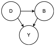
Total vs Direct effect
The direct effect of D on Y is the effect not mediated by anything else.
The total effect of D on Y is the effect including any mediators (like B).
Measuring direct effect would mean conditioning on B.
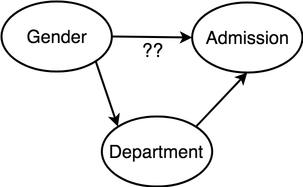
Berkley Admission Gender Bias
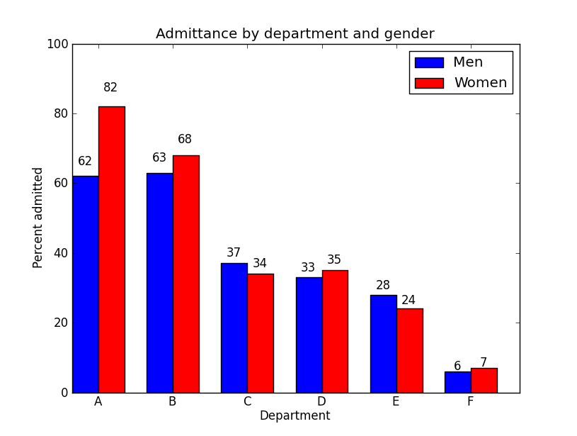
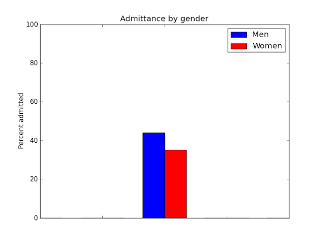
Gender influences both department and, possibly, admission.
What we are interested is the direct effect of gender on admission, not the total effect.
So conditioning by department is the right thing to do.
Berkley Admission Gender Bias
Testable implications
You can test your causal diagram. For example, according to this diagram:
u ⊥ b
u ⊥ c
a ⊥ c ∣ d
b ⊥ c ∣ d
Given a dataset, algorithms exist that can "prune" the space of potential causal models.
A/B testing
Random assignment to a certain group can be visualised in DAGs.
In the right represents on A/B test for a drug. Assignment to the drug has no causes, i.e., it is associated with nothing.
According the the backdoor criteria, we do not need to condition on anything.
DAG Parties
Never done it, but I heard of meetings / parties where domain experts build their causal DAG and discuss why. This aids in finding and rejecting DAGs.
Time varying
DAGS can also be represented with time varying components, typically discretised into steps.

How to control for confounders
Regression for inference
Regression is like cheating. It's a simple way to control for variables that are categorical, continuous, linear/non-linear, interactions, etc.*
Simplest model is a linear regression:
* caveats but not for this 101 intro
Regression for inference
After finding the optimal parameters, if our assumptions are correct (big if), we can make statements like "the causal effect of X on Y is beta, which is or is not significantly far from the null".
Table 2 Fallacy
Let us assume that we estimate the effect of X on Y. We know from a DAG that there is only one confounder, Z, so we run the regression Y~X+Z.
The coefficient of X estimates the causal effect of X on Y.
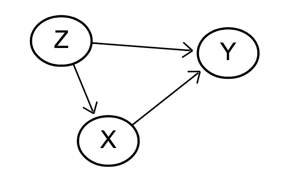
Table 2 Fallacy
The ‘Table 2 fallacy’ is the belief that we can also interpret the coefficient of Z as the effect of Z on Y;
In larger models, the fallacy is the belief that all coefficients have a similar interpretation with respect to Y.
Table 2 Fallacy
X mediates the effect of Z on Y, but adjustment for a mediator is wrong when estimating the total causal effect.
Table 2 Fallacy
X mediates the effect of Z on Y, but adjustment for a mediator is wrong when estimating the total causal effect.
The Z coefficient in our model cannot be interpreted as a total causal effect. Instead, we could interpret it as the direct effect of Z on Y; this could be stronger than, weaker than, or opposite to the total effect.
Table 2 Fallacy
In summary, some regression coefficients represent the total effect, and others the direct effect, and some have no causal interpretation at all.
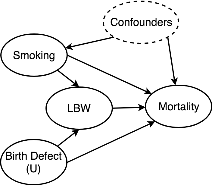
LBW Paradox
We can finally answer the LBW paradox.
Researchers can ask two questions:
LBW Paradox
We can finally answer the LBW paradox.
Researchers can ask two questions:
1. What is the direct effect of smoking on mortality?
LBW Paradox
We can finally answer the LBW paradox.
Researchers can ask two questions:
1. What is the direct effect of smoking on mortality?
2. What is the total effect of smoking on mortality?
LBW Paradox
What is the direct effect of smoking on mortality?
To answer this, we need to condition on LBW - but LBW is a collider with birth defects. That's okay, if we can control for birth defects, but unfortunately it's unobserved.
This causes a bias, and hence the paradox.
LBW Paradox
What is the total effect of smoking on mortality?
To answer this, we should not control for LBW. Simple as that. (We should however still control for the confounders)
LBW Paradox
"Adjusted" Model (direct effect)
"Raw" Model (total effect)
LBW Paradox
"Adjusted" Model (direct effect)
"Raw" Model (total effect)
| Model | beta_1 |
|---|---|
| "Adjusted" | 0.086 |
| "Raw" | 0.438 |
Shopify Examples
-
What's the impact of latency on checkout conversion
-
What is the causal impact of a merchant's first sale on retention?
-
What is the effect on shops sales of installing channel X, or app Y?
Tools
dagitty.net
statsmodels
lifelines
Zepid