Limiting shape for first-passage Percolation models

on random geometric graphs

Cristian F. Coletti (UFABC)

Overview

Introduction to First-passage percolation (FPP)

Random geometric graphs (RGG)

First-passage percolation

Asymptotic shape theorem

Richardson model

Overview

19/19056-2

20/12868-9

17/10555-0

Introduction to First-passage percolation (FPP)

Random geometric graphs (RGG)

First-passage percolation

Asymptotic shape theorem

Richardson model

Lucas R. de Lima (UFABC)

Joint work with

Daniel Valesin (Warwick)

Alexander Hinsen (WIAS - Berlin)

Benedikt Jahnel (WIAS - Berlin)

Supported by

What is it about?

first passage percolation on

Introduced by Hammersley and Welsh in 1965 as a model for the spread of a fluid.

Attach a nonnegative R.V. t(e) so that the (t(e) : e is and edge) is I.I.D.

t(e) is interpreted as a passage time (or time needed to cross e).

Define the shortest time to connect x to y by

\mathbb{Z}^d

T(x,y) = \inf \{\displaystyle \sum_{e \in \gamma : x \rightarrow y} t(e)\}

The infimum is over all paths connecting x to y. Recall that a path is a finite sequence of vertices and edges

(v_0,e_1,v_1,...,e_n,v_n)

such that

v_0=x, v_n=y, e_i=(v_{i-1},v_i).

FIRST-PASSAGE PERCOLATION

Time constant

It is of interest to study the asymptotic behavior of

T(0,nx).

Under some assumption on the distribution of t(e) we get

\displaystyle\lim_{n \rightarrow \infty} \frac{T(0,nx)}{n} = \mu(x) \ \ \ a.s. - L^1, x \in \mathbb{Z}^d

\text{when this limit exists and we call} \ \mu(e_1) \ \text{the time constant.}

Time constant

(T(nx,mx))_{1 \leq n \leq m}

Remark: This follows from the sub-additivity of the sequence

Idea: It follows from the translation invariance of the model that

\mathbb{E}[T(0,(n+m)x)] \leq \mathbb{E}[T(0,nx)] + \\ \mathbb{E}[T(0,mx)] \ \forall \ m,n \geq 1.

Time constant

Fekete´s lemma and finite first moment of

T(0,x)

guarantees that

\displaystyle \lim_{n \rightarrow +\infty} \frac{\mathbb{E}[T(0,nx)]}{n}

exists and it is finite. Name this limit

\mu(x)

Time constant

That

\displaystyle \lim_{n \rightarrow +\infty} \frac{T(0,nx)}{n} = \mu(x)

follows from Kingman´s - Liggett subadditive ergodic theorem applied to the sequence

\left(T(nx,mx) : 0 \leq n < m \right), \ \ \ x \in \mathbb{Z}^d .

Time constant

Remark: The time constant has been defined only for

x \in \mathbb{Z}^d.

Then extend the time constant to the whole space using

Remark: Kesten (1984) proved that we can use K-L theorem under the assumption

\bullet \ \text{The uniform continuity of the time constant on} \ \mathbb{Q}^d \ \text{and}

\bullet \ \text{The density of} \ \mathbb{Q}^d \ \text{on} \ \mathbb{R}^d .

Time constant

\mathbb{E}[\min\{t_1, \ldots, t_{2d}\}] < +\infty

where the R.V. in the minimum are i.i.d. copies of the passage time.

Kesten (1984) proved that the time constant is a norm in the whole space if and only if

\nu(\{0\}) < p_c(d) .

Then,

Time constant

Cox-Durrett (1981) proved that if conditions

\nu(\{0\}) < p_c(d)

and

\mathbb{E}[\min\{t^d_1, \ldots, t^d_{2d}\}] < +\infty

\left(1-\epsilon\right) \mathfrak{B} \subset \frac{1}{t} B(t) \subset \left(1+ \epsilon\right) \mathfrak{B} .

\text{hold, then for any} \ \epsilon > 0 \ \text{a.s} \ \exists M : \forall t \geq M

Time constant

\bullet \ \text{Indeed,} \ \mathfrak{B} \ \text{is the unit ball for the norm} \ \mu .

\bullet \ \text{Here,} \ B(t) \ \text{is the set of points that can be reached from}

\text{the origin by time} \ t. \ \text{(fattened version)}

FIRST-PASSAGE PERCOLATION

First-passage percolation

The model

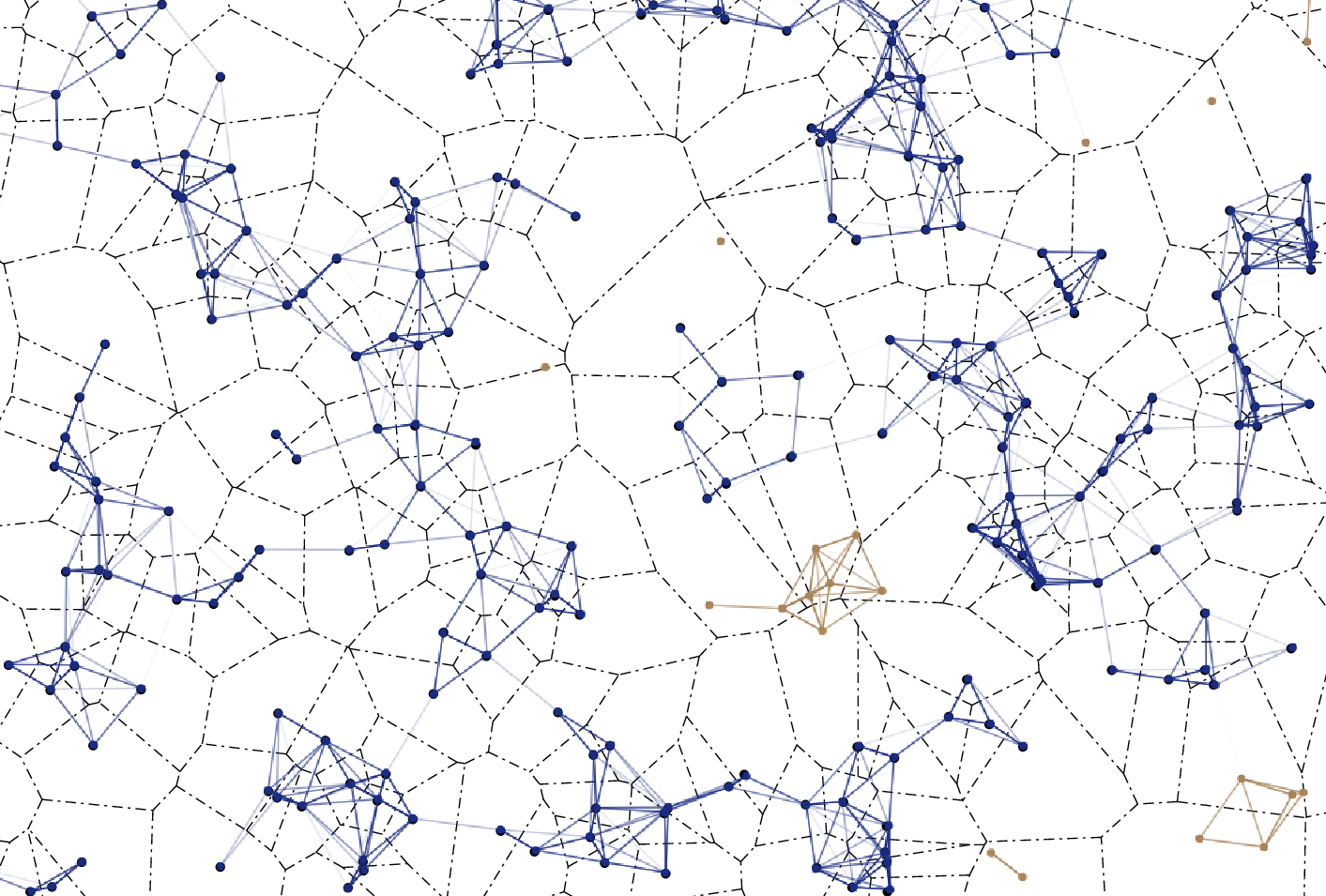
Random geometric graph

\text{Let} \ \mathcal{P}_\lambda \ \text{be the random set of points determined by} \\ \text{the homogeneous PPP on} \ \mathbb{R}^d \ \text{with intensity} \ \lambda>0.

\bullet \ \text{The RGG} \ \mathcal{G}_{\lambda,r}=(V,E) \ \text{on} \ \mathbb{R}^d \ \text{is defined by}

V = \mathcal{P}_\lambda \ \text{and} \ E = \big\{\{u,v\} \subseteq V: ||u-v|| < r , \ u \neq v\big\},

\ \ \text{where} \ ||\cdot|| \ \text{is the Euclidean norm.}

The model

Remark:

\bullet \ \text{We want to study the spread of an infection} \\ \text{on an infinite connected component of} \ \mathcal{G}_{\lambda , r}.

\bullet \ \text{For all} \ d \geq 2 \ \exists \ r_c(\lambda)>0 : \mathcal{G}_{\lambda , r} \ \text{has an infinite component}

\mathcal{H}, \ \textit{a.s.} \ \text{for all} \ r > r_c(\lambda) \ \text{which is} \ \textit{a.s.} \ \text{unique.}

The model

\bullet \ \mathcal{H} \ \text{is a subgraph of} \ \mathcal{G}_{\lambda , r}.

\bullet \ \ \text{Denote by} \ \left(V(\mathcal{H}), E(\mathcal{H})\right) \ \text{the resulting graph.}

\bullet \ \text{It is well known that} \ r_c (1) \geq 1/{\upsilon_d}^{1/d} \ \text{here} \ \upsilon_d \ \text{denotes}

\text{the volume of the} \ d-\text{dimensional unit ball.}

q(x)= \operatorname{arg~min}_{y\in V(\mathcal{H})} \|y-x\|

\text{Let us define for every} \ x \in \mathbb{R}^d

Existe

Voronoi partition

q \ \text{induces a Voronoi partition of} \ \mathbb{R}^d \ \text{with respect to} \ \mathcal{H} .

Voronoi partition

FIRST-PASSAGE PERCOLATION

We assign a random length

\tau_e \geq 0

to each edge

e \in E(\mathcal{H}).

Let

\{\tau_e\}_{e \in E(\mathcal{H})}

be independent and identically distributed with

\tau_e \sim \tau.

FIRST-PASSAGE PERCOLATION

We define the passage time between by the random variable

x,y \in \R^d

T(x,y) := \inf\left\{\sum_{e\in\gamma} \tau_{e}: \gamma\in\mathscr{P(q(x),q(y))}\right\}

FIRST-PASSAGE PERCOLATION

Let denote the random set of regions (Voronoi cells)

reached up to time t with the FPP starting from q(o).

H_t

H_t := \big\{ x \in \mathbb{R}^d: {T(o,x) \leq t} \big\}

Asymptotic shape theorem

Set

(A1)

\mathbb{P}(\tau = 0) < \dfrac{1}{(\upsilon_d r^d\lambda).} \quad;

(A2)

\mathbb{E}[\tau^\eta] < +\infty.

There exists

\eta > 2(d + 1)

such that

Asymptotic shape theorem

Let

d \geq 2

and

r > r_c

Then there exists
one has

\varphi > 0

such that, for all

\text{a.s.}

for

n \gg 1.

(1-\varepsilon)B(\varphi) \subseteq \frac{1}{n}H_n \subseteq (1+\varepsilon)B(\varphi)

. Consider i.i.d. FPP on a RGG

satisfying (A1) and (A2)

\varepsilon \in (0,1)

that

Sketch of the proof

The passage time grows at most linearly
The passage time grows at least linearly
We apply Kingman`s subadditive ergodic theorem

Shape

Consequence of the rotational invariance

At most linear growth

\mathbb{E}[T(o,x)] \geq a \|x\|

Condition (A1) implies that there exists such that

a>0

At Least linear growth

\mathbb{P}\Big(T(o,x) > t\Big) < c \cdot t^{-(d+\kappa)}.

Condition (A2) implies that there exist such that

for each and all , one has that

\beta,\kappa>1

x \in \mathbb{R}^d

t \geq \beta \|x\|

Subadditive ergodic theorem

\lim_{n\to\infty} \frac{T(o,nx)}{\|nx\|} = {\varphi}^{-1} \quad \text{a.s.}

(Kingman)

Asymptotic equivalence

\lim\limits_{\|x\|\to+\infty}\dfrac{T(o,x)}{\|x\|} = {\varphi}^{-1} \quad \text{a.s.}

Existence of the limiting shape

Simulation of the Richardson's infection model

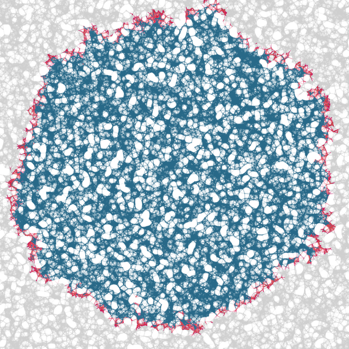
Richardson's growth model (1973)

\bullet \ \text{At} \ t \geq 0, \ \text{a site of} \ \mathcal{H} \ \text{is either } \ \text{healthy (0) or infected (1). }

\bullet \ \zeta_t:V(\mathcal{H})\to \{0,1\} \ \text{denotes the state of the sites at time t}

\bullet \ \text{Model the spread of an infection (growth of a population).}

RICHARDSON'S GROWTH MODEL

\bullet \ \text{The process evolves as follows:}

\bullet \ \text{A healthy particle becomes infected at rate}

\lambda_{I}\sum_{y \sim x}\zeta_t(y).

\bullet \ \text{An infected particle remains infected forever.}

RICHARDSON'S GROWTH MODEL

\bullet \ \text{The process is determined by FPP with edge passage times}

\tau_e \sim \mathrm{Exp}(\lambda_{I})

\text{independently for each} \ e \in E(\mathcal{H}).

RICHARDSON'S GROWTH MODEL

\bullet \ \text{Condition} \ (A_1) \ \text{is straightforward since}

\bullet \ \text{Condition} (A_2) \ \text{holds since}

\mathbb{P}(\tau=0)=0<1/(\upsilon_d r^d\lambda).

\ \mathbb{E}[\exp(\alpha\tau)] < +\infty \ \text{for} \ \alpha \in (0, \lambda_{r I}).

RICHARDSON'S GROWTH MODEL

\bullet \ \text{The shape theorem holds for the Richardson model on} \ \mathcal{H}

\text{for any} \ r > r_c(\lambda).

Thank you!

Preprint available on

arxiv:2109.07813

Time-space rescaling for Richardson model

\bullet \ \text{Asymptotic behavior of the Richardson model}

\bullet \ \text{The limiting process is a branching process}

(\mathcal{T}^{\lambda,\lambda_{I}}_t)_{t\geq 0}.

\text{The limit object}

\bullet \ \mathcal{T}^{\lambda,\lambda_{I}}_0=o.

TIME-SPACE RESCALING FOR RICHARDSON MODEL

\bullet \ \text{Offsprings are given by PPP}(\upsilon_d r^d\lambda\lambda_{I}) \ \text{ (time)}

\bullet \ \text{Offsprings are placed independently and uniformly within}

B_r(X_i).

TIME-SPACE RESCALING FOR RICHARDSON MODEL

\text{Let} \ r > r_{c}(\lambda). \ \text{Then,}

\mathcal{H}_{[0,t]}^{\alpha \lambda, \lambda_{I}/\alpha} \longrightarrow \mathcal{T}^{\lambda, \lambda_{I}}_{[0,t]}

\text{weakly with respect to the Skorokhod topology, as }

\alpha \rightarrow \infty

TIME-SPACE RESCALING FOR RICHARDSON MODEL

Remark:

\text{The subscript} \ [0,t] \ \text{indicates that we consider the whole path from}

\ 0 \ \text{to} \ t.

Ongoing work

Lucas R. de Lima, D. Valesin, C. F. C.

\bullet \ \text{Quantitative shape theorem for FPP on RGG}

\bullet \ \text{Moderate deviation for the passage time}

\bullet \ \text{A dynamic on RGGs}