Autoenconders
Cristóbal Silva
What's an Autoencoder?
Encoder
Decoder
Low Dimensional
Representation
Input
Output
Just an MLP where
input size = output size
Advantages
- Undercomplete representation forces algorithm to learn most important features
- Can be transferred to other domains once it has been trained
- Can be used as generative models under certain conditions
Tying Weights
Encoder
Transposed Encoder
Low Dimensional
Representation
Input
Output
Half the parameters!
Tying Weights
import tensorflow as tf
w_encode_1 = tf.Variable(w_encode_1_init, dtype=tf.float32)
w_encode_2 = tf.Variable(w_encode_2_init, dtype=tf.float32)

w_decode_2 = tf.transpose(w_encode_2)  # tied weights
w_decode_1 = tf.transpose(w_encode_1)  # tied weights
Tensorflow
from torch.autograd import Variable
w_encode_1 = Variable(w_encode_1_init)
w_encode_2 = Variable(w_encode_2_init)

w_decode_2 = w_encode_2.t()  # tied weights
w_decode_1 = w_encode_1.t()  # tied weights

# alternative
def forward(self, x):
    x = self.encode_1(x)
    x = self.encode_2(x)
    x = F.linear(x, weight=self.encode_1.weight.t())  # tied weights
    x = F.linear(x, weight=self.encode_2.weight.t())  # tied weights
    return x
PyTorch
Note: biases are never tied, nor regularized
Denoising Autoencoders
Encoder
Decoder
Low Dimensional
Representation
Corrupted Input
Clean Output
Better reconstruction!
What is corruption?
Adding noise
Shutting down nodes
Denoising autoencoder prevents neurons from colluding with each other, i.e. it forces each neuron or a small group of neurons to do its best in reconstructing the input
Sparse Autoencoders
Encoder
Decoder
Low Dimensional
Representation
Input
Output
Efficient representation!
Why Sparsity?
- Force the least amount of nodes per activation for compact representation
- Each neuron in the hidden layers represents a useful feature
- Requires to compute the average activation in the coding layer over the training batch (*)
(*): Avoid small batches, or the mean will not be accurate
Sparsity Loss
def kl_divergence(p, q):
    return p * tf.log(p / q) + (1 - p) * tf.log((1 - p) / (1 - q))

reconstruction_loss = tf.reduce_mean(tf.square(outputs - X))  # MSE
sparsity_loss = tf.reduce_sum(kl_divergence(sparsity_target, hidden_mean))
loss = reconstruction_loss + sparsity_weight * sparsity_loss
Variational Autoencoders
Encoder
Decoder
Input
Output
Generative model!
Low Dimensional
Representation
Latent Loss
Penalizing this term ensures that the codings are close to a unit-gaussian.
This is useful because we only need to sample from \( \mathcal{N}(0, 1) \) and pass through the decoder network to generate from \( P(X|z) \)
Applications in HSI
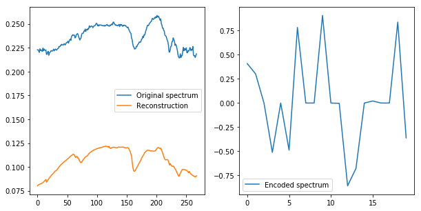
Stacked Autoencoder
References


https://github.com/ageron/handson-ml/blob/master/15_autoencoders.ipynb
https://github.com/GunhoChoi/Kind-PyTorch-Tutorial