Generative Adversarial Nets
Cristóbal Silva
Why GANs
- Simulate Future
- Work with missing data
- Multi-modal outputs
- Realistic generation tasks

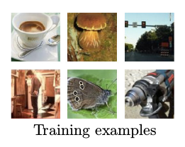
Maximum Likelihood
in Deep Learning
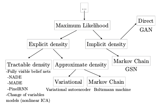
sample without density
GANs
- Latent code
- Asymptotically consistent
- No Markov Chains needed
- (Subjective) Produces bests samples
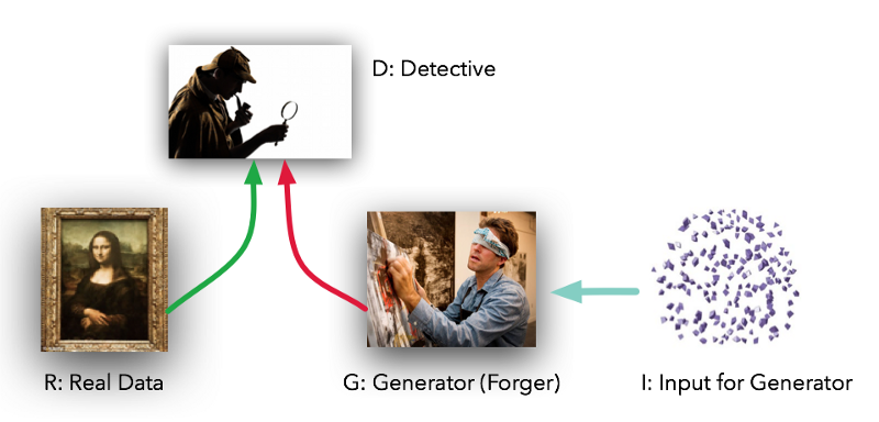
Generator vs Discriminator
Generator vs Discriminator
D(x) = \text{discriminator}
G(z) = \text{generator}
z = \text{noise input}
X = \text{training data}
p_{generator}(x)
p_{data}(x)
0: real

1: fake
Nash Equilibrium
p_{data}(x) = p_{generator}(x)
D(x) = \frac{1}{2}
In other words, discriminator can't discriminate
Loss Function
Minimax Game
J^{(D)} = -\frac{1}{2}\mathbb{E}_{\mathbf{x}\sim p_{data}} \log{D(\mathbf{x})} - \frac{1}{2}\mathbb{E}_{\mathbf{z}} \log{(1 - D(G(\mathbf{z}))}
J^{(G)} = -J^{(D)}
Non-Saturating Game
J^{(D)} = -\frac{1}{2}\mathbb{E}_{\mathbf{x}\sim p_{data}} \log{D(\mathbf{x})} - \frac{1}{2}\mathbb{E}_{\mathbf{z}} \log{(1 - D(G(\mathbf{z}))}
J^{(G)} = -\frac{1}{2}\mathbb{E}_{\mathbf{z}} \log{D(G(\mathbf{z}))}
Vanishing gradient
GANs + PyTorch,
Let's model and sample from a Gaussian!
import torch
import torch.nn as nn
import torch.nn.functional as F
import torch.optim as optim
PyTorch is a new DL framework based on dynamic graphs
Comes with high level API for network design
No static-graph required, easier to debug
What we need
Input data
Input noise
our ground truth
our latent code
def real_distribution_sampler(mu, sigma, n):
    samples = np.random.normal(mu, sigma, (1, n))
    return torch.Tensor(samples)
def noise_distribution_sampler(m, n):
return torch.rand(m, n)Generator
class Generator(nn.Module):
    def __init__(self):
        super().__init__()
        self.fc1 = nn.Linear(1, 100)
        self.fc2 = nn.Linear(100, 100)
        self.fc3 = nn.Linear(100, 1)

    def forward(self, x):
        x = F.elu(self.fc1(x))
        x = F.sigmoid(self.fc2(x))
        x = self.fc3(x)
        return x
class Discriminator(nn.Module):
def __init__(self):
super().__init__()
self.fc1 = nn.Linear(100, 50)
self.fc2 = nn.Linear(50, 50)
self.fc3 = nn.Linear(50, 1)
def forward(self, x):
x = F.elu(self.fc1(x))
x = F.elu(self.fc2(x))
x = F.sigmoid(self.fc3(x))
return xDiscriminator
1
100
100
1
100
1
50
50
Training
Parameters
Optimization
n_epochs = 30000

# binary cross entropy loss
criterion = nn.BCELoss()

# discriminator params
D = Discriminator()
d_steps = 1
d_optimizer = optim.SGD(
               D.parameters(),
               lr=2e-4
              )


# generator params
G = Generator()
g_steps = 1
g_optimizer = optim.SGD(
               G.parameters(),
               lr=2e-4
              )
batch_size = 100
for epoch in range(n_epochs)
    for i in range(d_steps):
        D.zero_grad()
        # train D on real data
        d_real_data   = Variable(real_distribution_sampler(mu, sigma, 100))
        d_real_output = D(d_real_data)
        d_real_loss   = criterion(d_real_output, Variable(torch.ones(1)))
        d_real_loss.backward()  # compute/store gradients, but don't update

        # train D on fake data
        d_gen_input   = Variable(noise_distribution_sampler(batch_size, 1))
        d_fake_data   = G(d_gen_input).detach()  # important to avoid training G
        d_fake_output = D(d_fake_data.t())
        d_fake_loss   = criterion(d_fake_output, Variable(torch.zeros(1)))
        d_fake_loss.backward()

        d_optimizer.step()

    for j in range(g_steps):
        # train G based on D output
        G.zero_grad()
        g_gen_input   = Variable(noise_distribution_sampler(batch_size, 1))
        g_fake_data   = G(g_gen_input)
        g_fake_output = D(g_fake_data.t())
        g_fake_loss   = criterion(g_fake_output, Variable(torch.ones(1)))
        g_fake_loss.backward()
        g_optimizer.step()
Experiment

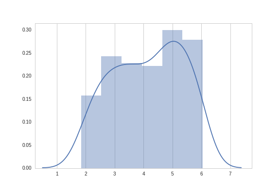
| mean | 4.00 |
| var | 1.25 |
SGD
Results 1
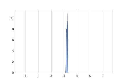
| mean | 4.00 |
| var | 1.25 |
| mean | 4.21 |
| var | 0.03 |
... the dreaded mode-collapse!
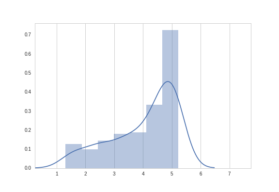
SGD
Results 2
| mean | 4.00 |
| var | 1.25 |
| mean | 3.82 |
| var | 1.13 |
SGD with Momentum
Results 3
| mean | 4.00 |
| var | 1.25 |
| mean | 4.26 |
| var | 1.09 |
ADAM
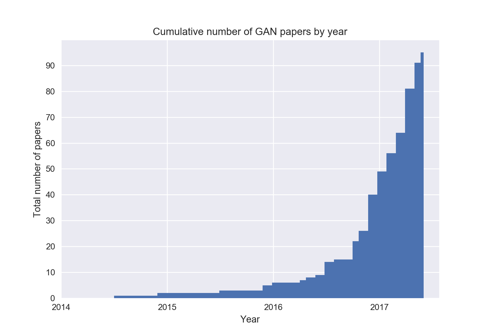
GAN Zoo
What we saw was 2 years ago, what now?
Many, many GANs
ose-GAN


enderGAN

AD-GAN

riple-GAN

nrolled GAN

AE-GAN

aterGAN
A

B

C

D

E

F

G

H

I

J

K

L

M
N

O

P

Q

R

S

T

U

V

W

X

Y

Z
daGAN

ayesian GAN

atGAN

CGAN

BGAN

-GAN

eneGAN

yperGAN

GAN


AGAN

cGAN
More than 90 papers in 2017
DCGAN
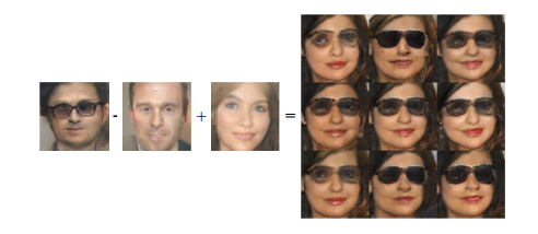
GANs can encode concepts

pix2pix
DiscoGAN

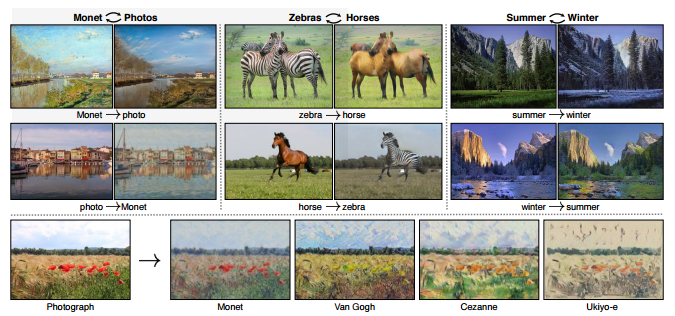
Cycle-GANs
Problems
- Classical GANs generate from input noise. This means you can't select the features you want the sample to have
- If you wanted to generate a picture with specific features, there's no way of determining which initial noise values would produce that picture, other than searching over the entire distribution.