Soss: Lightweight Probabilistic Programming in Julia

Chad Scherrer

Senior Data Scientist, Metis

About Me

Served as Technical Lead for language evaluation for the DARPA program
Probabilistic Programming for Advancing Machine Learning (PPAML)

PPL Publications

Scherrer, Diatchki, Erkök, & Sottile, Passage : A Parallel Sampler Generator for Hierarchical Bayesian Modeling, NIPS 2012 Workshop on Probabilistic Programming
Scherrer, An Exponential Family Basis for Probabilistic Programming, POPL 2017 Workshop on Probabilistic Programming Semantics
Westbrook, Scherrer, Collins, and Mertens, GraPPa: Spanning the Expressivity vs. Efficiency Continuum, POPL 2017 Workshop on Probabilistic Programming Semantics

Making Rational Decisions

Managed Uncertainty

Rational Decisions

Bayesian Analysis

Probabilistic Programming

Physical systems
Hypothesis testing
Modeling as simulation

Medicine
Finance
Insurance

Risk

Custom models

Business Applications

https://cscherrer.github.io/post/max-profit/

Missing Data

The Two-Language Problem

A disconnect between the "user language" and "developer language"

Python

C

Deep Learning Framework

Harder for beginner users
Barrier to entry for developers
Limits extensibility

A New Approach in Julia

Give an easy way to specify models
Code generation for each (model, type of data, inference primitive)
Composability

A (Very) Simple Example

P(\mu,\sigma|x)\propto P(\mu,\sigma)P(x|\mu,\sigma)

\begin{aligned} \mu &\sim \text{Normal}(0,5)\\ \sigma &\sim \text{Cauchy}_+(0,3) \\ x_j &\sim \text{Normal}(\mu,\sigma) \end{aligned}

Theory

Soss

julia> Soss.sourceLogpdf()(m)
quote
    _ℓ = 0.0
    _ℓ += logpdf(Normal(0, 5), μ)
    _ℓ += logpdf(Normal(μ, σ), σ)
    _ℓ += logpdf(Normal(μ, σ) |> iid(N), x)
    return _ℓ
end

m = @model N begin
    μ ~ Normal(0,5)
    σ ~ Normal(μ,σ)
    x ~ Normal(μ,σ) |> iid(N)
end;

A Simple Linear Model

m = @model x begin
    α ~ Cauchy()
    β ~ Normal()
    σ ~ HalfNormal()
    yhat = α .+ β .* x
    y ~ For(eachindex(x)) do j
        Normal(yhat[j], σ)
    end
end

julia> m(x=truth.x)
Joint Distribution
    Bound arguments: [x]
    Variables: [σ, β, α, yhat, y]

@model x begin
        σ ~ HalfNormal()
        β ~ Normal()
        α ~ Cauchy()
        yhat = α .+ β .* x
        y ~ For(eachindex(x)) do j
                Normal(yhat[j], σ)
            end
    end

Observed data is not specified yet!

Sampling from the Posterior Distribution

julia> post = dynamicHMC(m(x=truth.x), (y=truth.y,)) |> particles
(σ = 2.02 ± 0.15, β = 2.99 ± 0.19, α = 0.788 ± 0.2)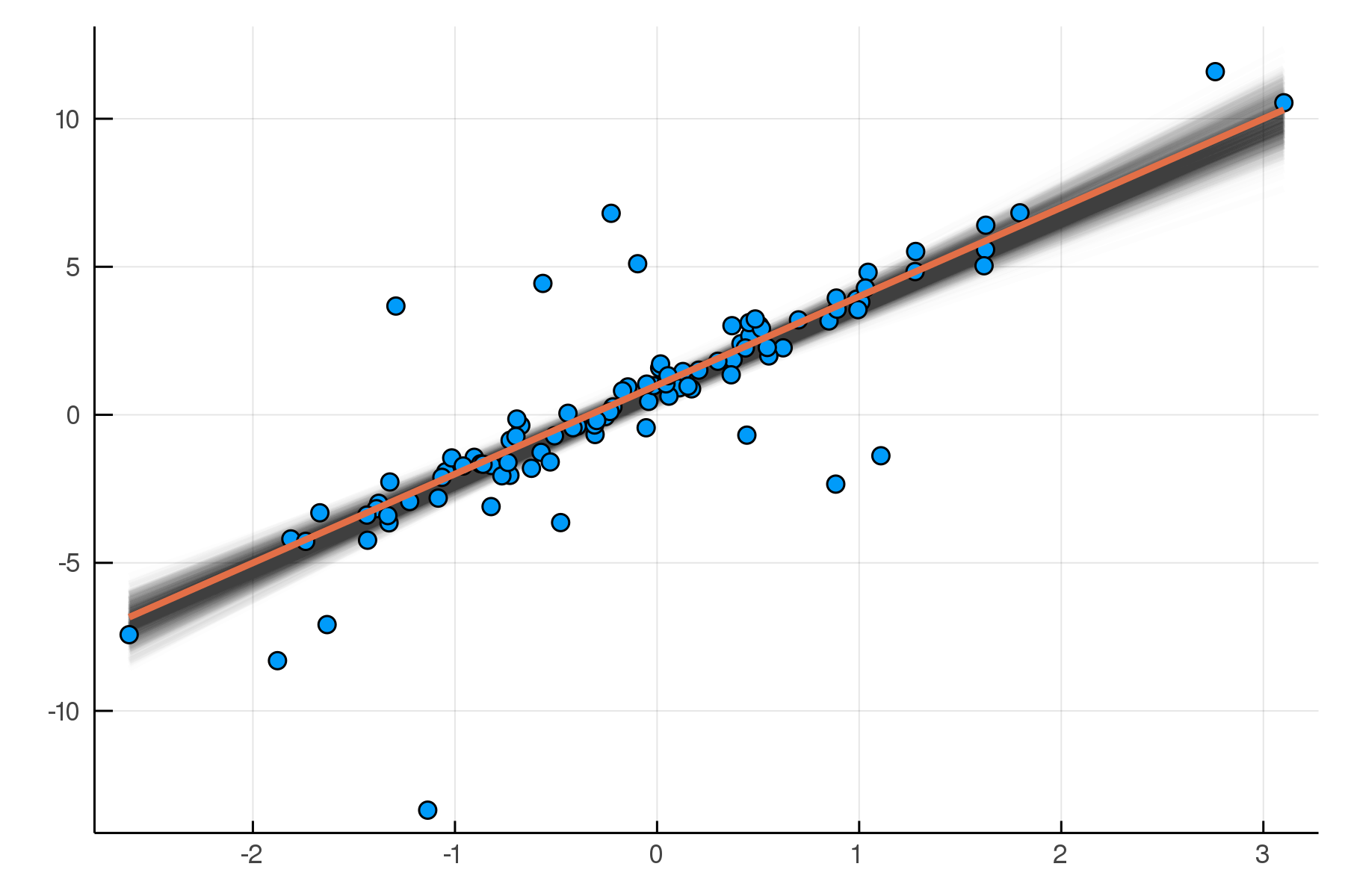

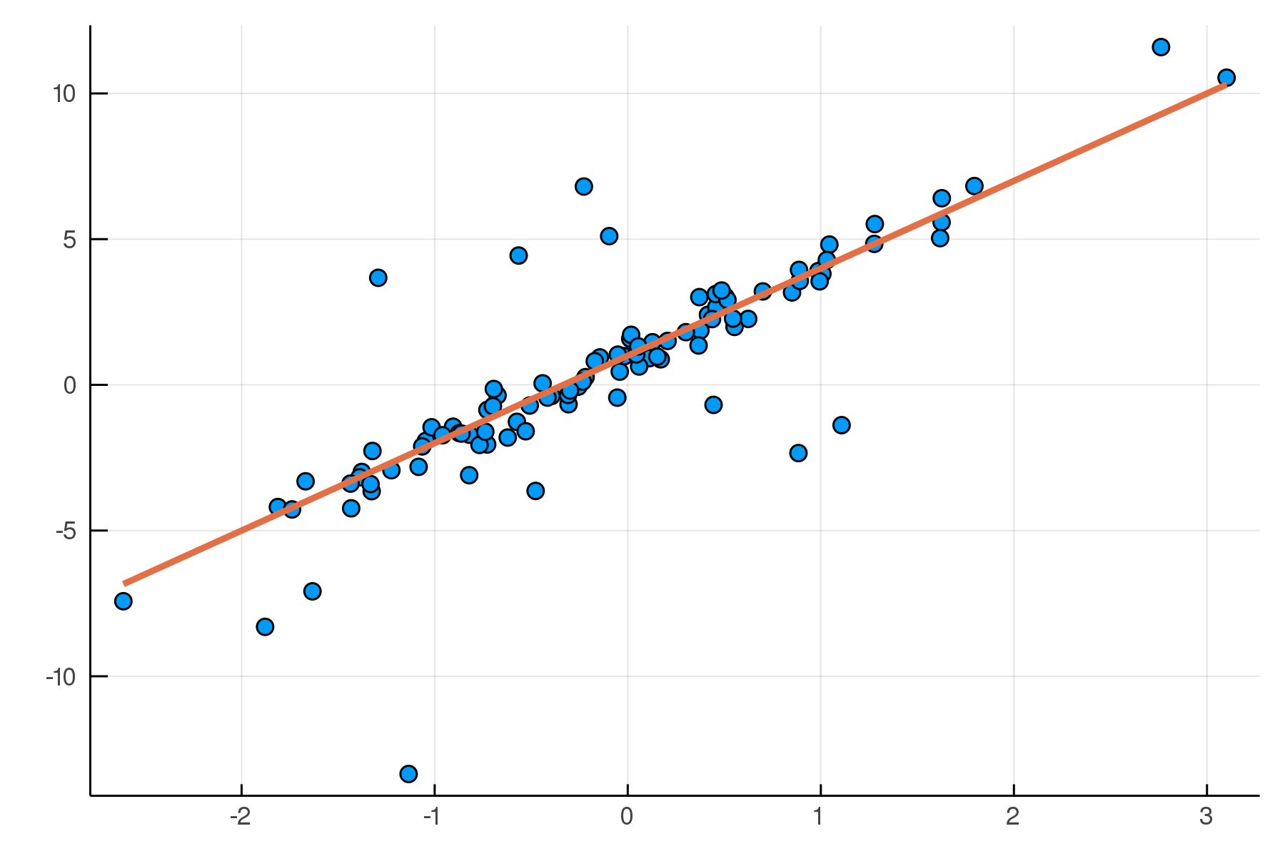
Posterior distribution

Possible best-fit lines

The Posterior Predictive Distribution

Start with Data

Sample Parameters|Data

Sample Data|Parameters

Real Data

Replicated Fake Data

Compare

Posterior

Distribution

Predictive

Distribution

The Posterior Predictive Distribution

julia> pred = predictive(m, :α, :β, :σ)
@model (x, α, β, σ) begin
    yhat = α .+ β .* x
    y ~ For(eachindex(x)) do j
            Normal(yhat[j], σ)
        end
end

m = @model x begin
    α ~ Cauchy()
    β ~ Normal()
    σ ~ HalfNormal()
    yhat = α .+ β .* x
    y ~ For(eachindex(x)) do j
        Normal(yhat[j], σ)
    end
end

postpred = [pred(θ)((x=x,)) for θ ∈ post] .|> rand |> particles

predictive makes a new model!

posterior predictive distributions

draw samples

convert to particles

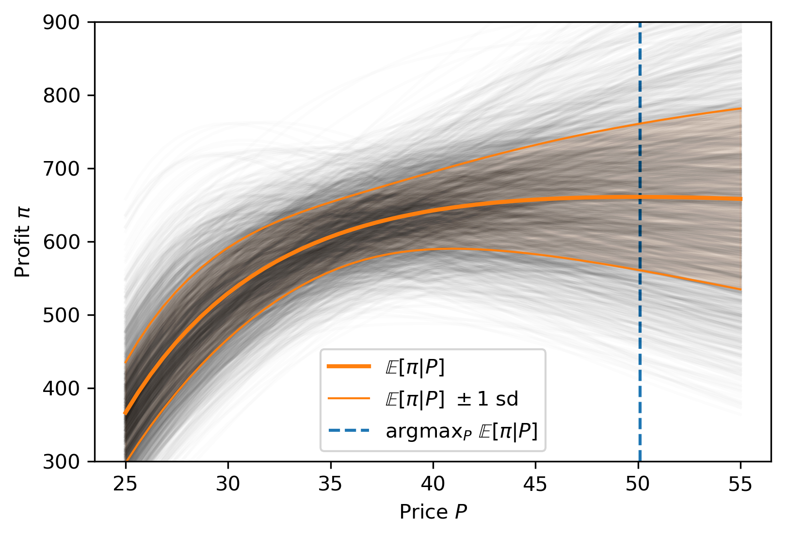
Posterior Predictive Checks

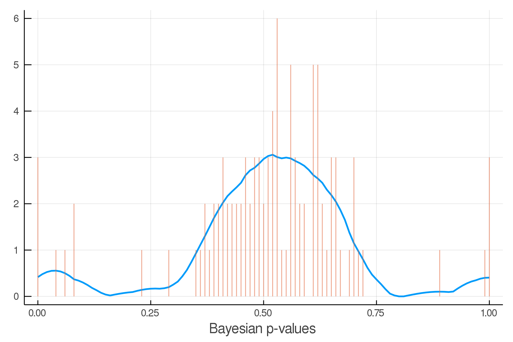
pvals = mean.(truth.y .> postpred.y)

Where we expect the data

Where we see the data

Making it Robust

m2 = @model x begin
    α ~ Cauchy()
    β ~ Normal()
    σ ~ HalfNormal(10)
    νinv ~ HalfNormal()
    yhat = α .+ β .* x
    y ~ For(eachindex(x)) do j
        StudentT(1/νinv,yhat[j],σ)
    end
end;

julia> post2 = dynamicHMC(m2(x=truth.x), (y=truth.y,)) |> particles
(σ = 0.444 ± 0.065, νinv = 0.807 ± 0.15
, β = 3.07 ± 0.064, α = 0.937 ± 0.062)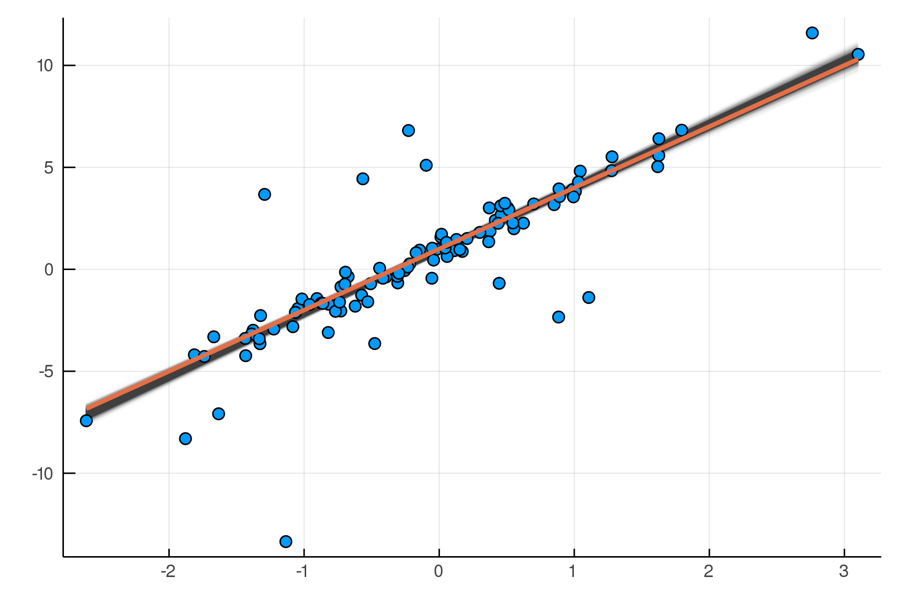

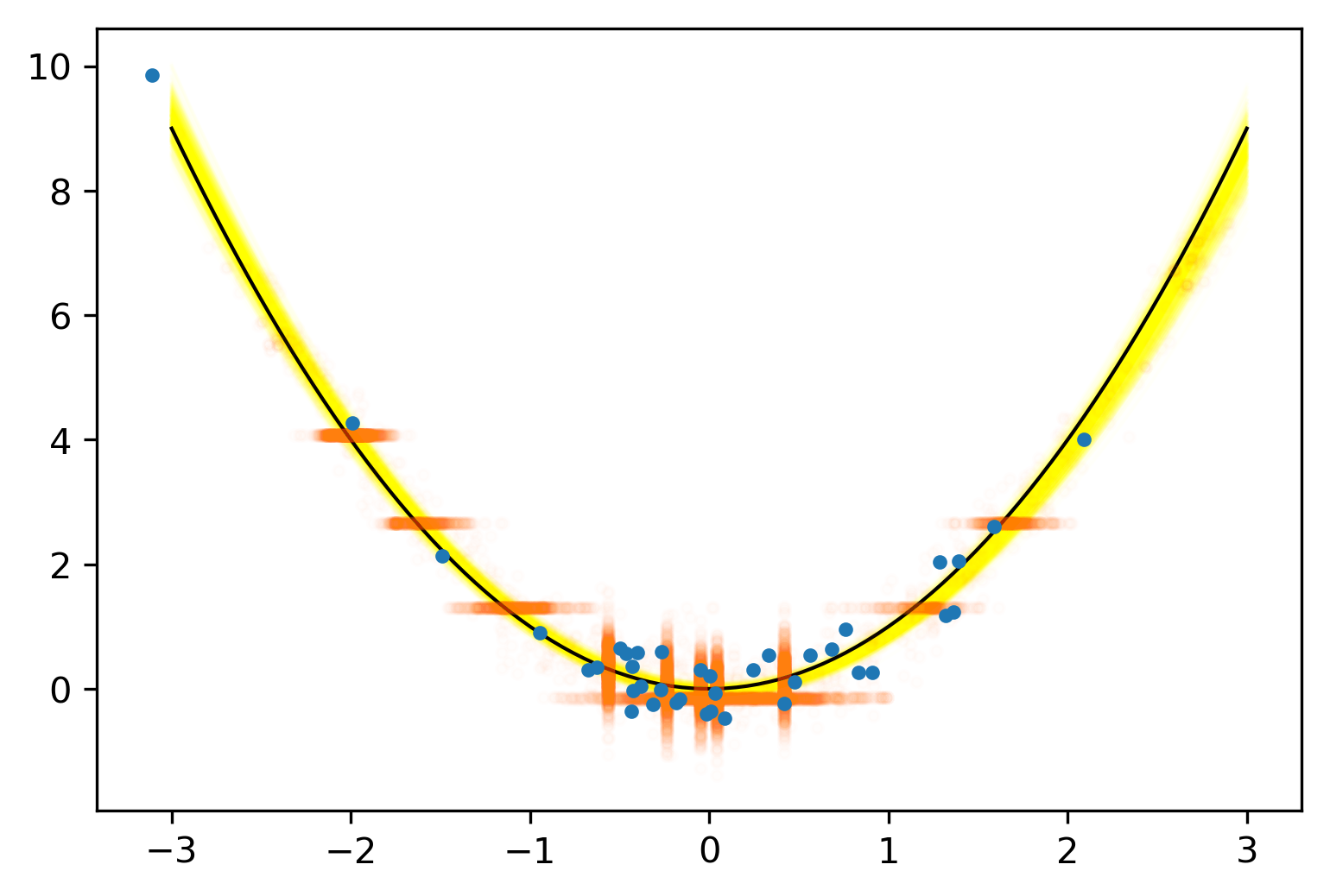
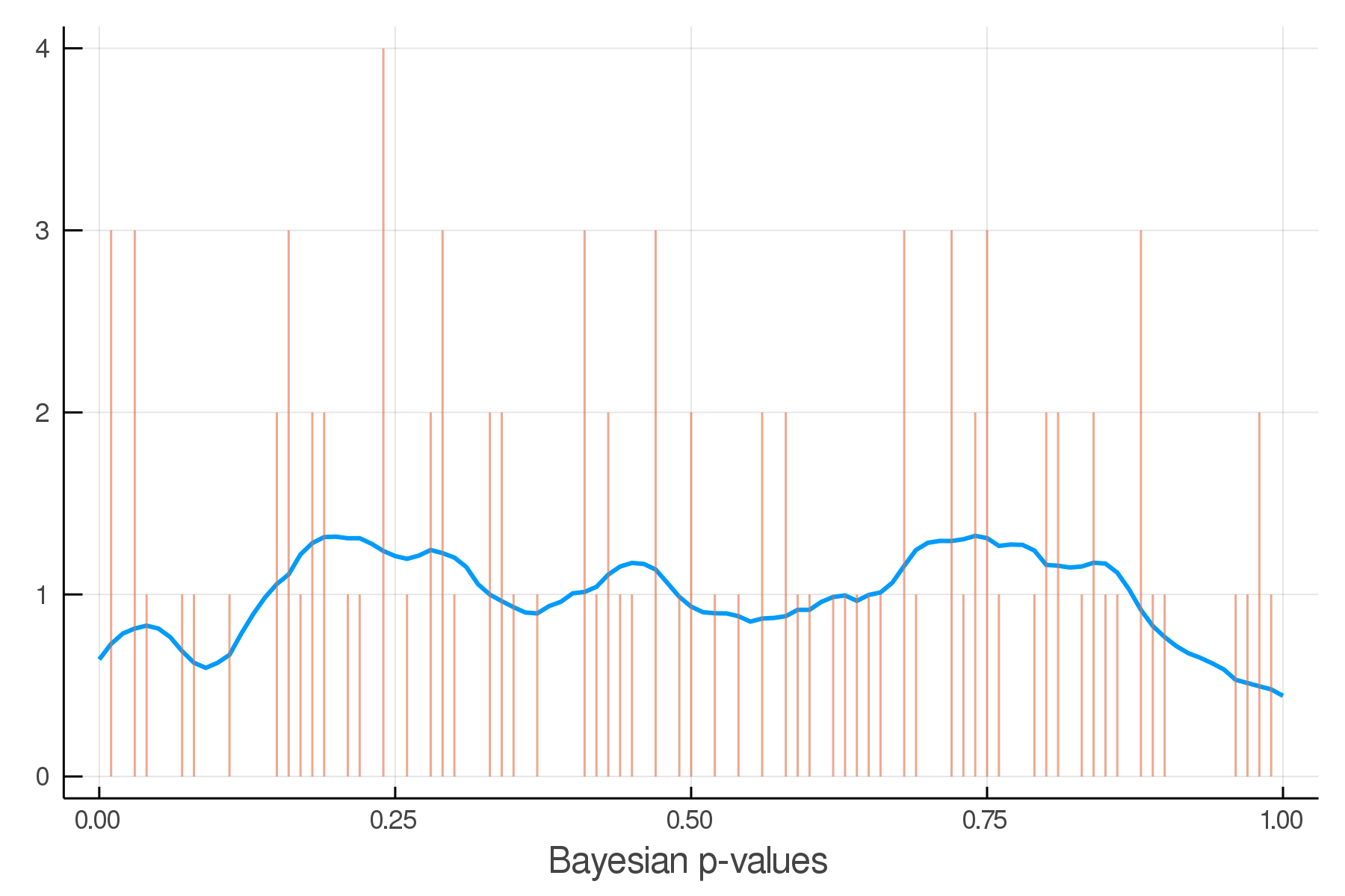
Updated Posterior Predictive Checks

Architecture Overview

Inference Primitives

xform, rand, particles, logpdf, weightedSample

Inference Algorithms

stream(sampler, myModel(args), data)

Stream Combinators

Rejection sampling
Approximate Bayes (ABC)
Expectation

Inference Primitive: rand

julia> Soss.sourceRand()(m)
quote
    σ = rand(HalfNormal())
    β = rand(Normal())
    α = rand(Cauchy())
    yhat = α .+ β .* x
    y = rand(For(((j,)->begin
            Normal(yhat[j], σ)
        end), eachindex(x)))
    (x = x, yhat = yhat, α = α
    , β = β, σ = σ, y = y)
end

m = @model x begin
    α ~ Cauchy()
    β ~ Normal()
    σ ~ HalfNormal()
    yhat = α .+ β .* x
    y ~ For(eachindex(x)) do j
        Normal(yhat[j], σ)
    end
end

Inference Primitive: logpdf

julia> Soss.sourceLogpdf()(m)
quote
    _ℓ = 0.0
    _ℓ += logpdf(HalfNormal(), σ)
    _ℓ += logpdf(Normal(), β)
    _ℓ += logpdf(Cauchy(), α)
    yhat = α .+ β .* x
    _ℓ += logpdf(For(eachindex(x)) do j
              Normal(yhat[j], σ)
          end, y)
    return _ℓ
end

m = @model x begin
    α ~ Cauchy()
    β ~ Normal()
    σ ~ HalfNormal()
    yhat = α .+ β .* x
    y ~ For(eachindex(x)) do j
        Normal(yhat[j], σ)
    end
end

First-Class Models

julia> m = @model begin
           a ~ @model begin
               x ~ Normal()
           end
       end;

julia> rand(m())
(a = (x = -0.20051706307697828,),)

julia> m2 = @model anotherModel begin
           y ~ anotherModel
           z ~ anotherModel
           w ~ Normal(y.a.x / z.a.x, 1)
       end;

julia> rand(m2(anotherModel=m)).w
-1.822683102320004

Coming Soon

\sum_j\left(a + b x_j\right) \rightarrow Na + b \sum_j x_j

Stream combinators via Transducers.jl and OnlineStats.jl
Connection to other PPLs: Turing.jl, Gen.jl
Normalizing flows with Bijectors.jl
Deep learning with Flux.jl
Gaussian processes
Symbolic simplification

Thank You!

https://cscherrer.github.io/

https://github.com/cscherrer/Soss.jl

julia-vscode

MonteCarloMeasurements.jl

Special Thanks for

AverageShiftedHistograms.jl