Eosam2024Tutorial
This is a live streamed presentation. You will automatically follow the presenter and see the slide they're currently on.
This is a live streamed presentation. You will automatically follow the presenter and see the slide they're currently on.
Giovanni Pellegrini
Data analysis
Direct model
Inverse model
These slides
Jahan, T. et al. Deep learning-driven forward and inverse design of nanophotonic nanohole arrays: streamlining design for tailored optical functionalities and enhancing accessibility. Nanoscale (2024) doi:10.1039/D4NR03081H.
| n.1 | n.2 | n.3 | |
|---|---|---|---|
| Lattice | Hexagonal | Square | Square |
| Material | Ag | Au | SiOx |
| Thickness (nm) | 100 | 115 | 90 |
| Radius (nm) |
60 | 110 | 140 |
| Pitch (nm) |
450 | 550 | 515 |
Jahan, T. et al. Deep learning-driven forward and inverse design of nanophotonic nanohole arrays: streamlining design for tailored optical functionalities and enhancing accessibility. Nanoscale (2024) doi:10.1039/D4NR03081H.
\( g_{_{W}}:\mathbb{R}^{n} \to \mathbb{R}^{m} \)
\( W \to \) neural network parameters (Weights)
\( g_{_{W}} \to \) differentiable everywhere
Input: \( x \in \mathbb{R}^{n} \)
Output: \( y \in \mathbb{R}^{m} \)
Weights: \( W_{i} = w^{i}_{jk} \)
Activation functions: \( f \)
\( z_{1} = W_{1} x \)
\( a_{1} = f^{1}(z_{1}) \)
\( \Downarrow \)
\( z_{l} = W_{l} a_{l-1} \)
\( a_{l} = f^{l}(z_{l}) \)
\( \Downarrow \)
\( y = f^{L}(z_{L}) \)
ReLU \[ f(x)=max\{0,x\} \]
Sigmoid \[ f(x)=\frac{1}{1 + e^{-x}} \]
GELU \[ f(x)=x * \Phi(x) \]
Input Data
SUPERVISED
LEARNING
Program
Output Data
TRADITIONAL
PROGRAMMING
Input Data
\( x \in \mathbb{R}^{n}\)
Output Data
\( y \in \mathbb{R}^{m}\)
Program
stored in \( w^{i}_{jk}\)
\[ Loss = \mathcal{L}(g_{_{W}}(x),y) \]
\[\mathcal{L}(g_{_{W}}(x),y) = \frac{1}{n} \sum _{i}^{batch} \lvert \lvert g_{_{W}}(x_{i}) - y_{i} \rvert \rvert_{1} \]
\[\mathcal{L}(g_{_{W}}(x),y) = \frac{1}{n} \sum _{i}^{batch} \lvert \lvert g_{_{W}}(x_{i}) - y_{i} \rvert \rvert_{2} \]
\[\mathcal{L}(g_{_{W}}(x),y) = \frac{1}{n} \sum _{i}^{batch} CE(g_{_{W}}(x_{i}) - y_{i}) \]
Mean Absolute Error
Mean Square Error
Cross Entropy
Thanks Jacopo !!!
| Lattice | Hexagonal |
| Material | Ag |
| Thickness (nm) | 100 |
| Radius (nm) |
60 |
| Pitch (nm) |
450 |
Direct: \( g_{_{W}}:\mathbb{R}^{5} \to \mathbb{R}^{200} \)
Inverse: \( g_{_{W}}:\mathbb{R}^{200} \to \mathbb{R}^{5} \)
# Loading the relevant libraries
import numpy as np  # numpy
import pandas as pd  # manipulation of tabular data
import matplotlib.pylab as plt # data plottingCredits: Alberto De Giuli
# Loading data
df = pd.read_csv('../DL-Assisted-NHA-Inverse-Design-/Dataset 6655.csv')  #load csv in dataframe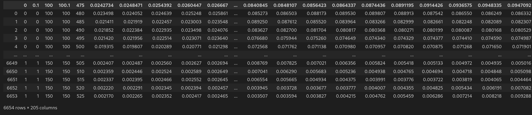
df # display dataframe in notebook# Loading data
filename = '../DL-Assisted-NHA-Inverse-Design-/Dataset 6655.csv' # define filename
df = pd.read_csv(filename) #load csv in dataframe
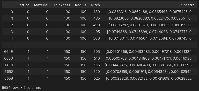
df # display dataframe in notebook# Formatting the data
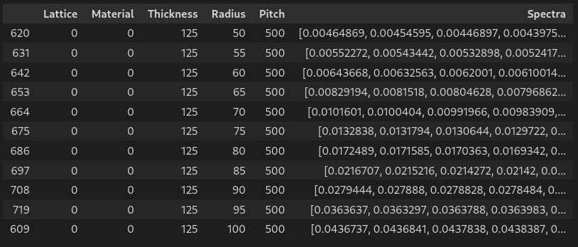
df['Spectra'] = df.values[:,5:][:,::-1].tolist() # gather 200 spectra column in one single list
df['Spectra'] = df['Spectra'].apply(np.array) # list to numpy array
df.drop(df.columns[5:-1], axis=1, inplace=True) # drop the gathered columns
df.columns = ['Lattice','Material','Thickness','Radius','Pitch','Spectra'] # name all columns
df # display dataframe in notebook# Inspecting the data for unique values
df['Lattice'].sort_values().unique()
df['Material'].sort_values().unique()
df['Thickness'].sort_values().unique()
df['Radius'].sort_values().unique()
df['Pitch'].sort_values().unique()# Unique values
array([0, 1]) # Lattice
array([0, 1, 2]) # Material
array([100, 105, 110, 115, 120, 125, 130, 135, 140, 145, 150]) # Thickness
array([ 50, 55, 60, 65, 70, 75, 80, 85, 90, 95, 100, 105, 110, 115, 120, 125, 130, 135, 140, 145, 150]) # Radius
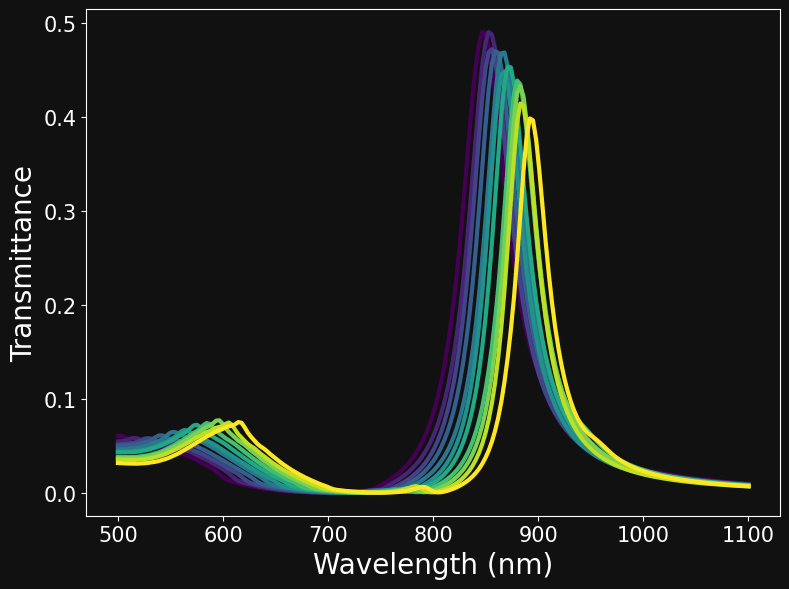
array([475, 480, 485, 490, 495, 500, 505, 510, 515, 520, 525]) # Pitch# create vector for wavelengths
wl_min, wl_max, n_wl = 500.0, 1100.0, 200
wavelengths = np.linspace(wl_min,wl_max,n_wl)
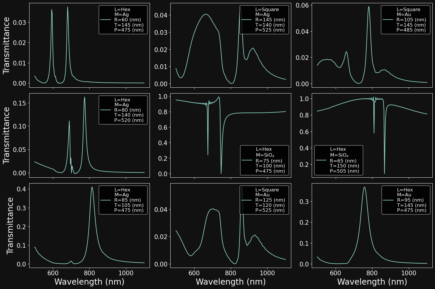
# create figure canvas
fig,axs = plt.subplots(3,3,figsize = (15,10),sharex=True,sharey=False)
# pick 9 random samples
samples = np.random.randint(0,6553,9)
# loop over the plot 3x3 grid
for i in range(3):
for j in range(3):
# create legend string depending on parameters
legend_str = 'L=' + str(lattices[df['Lattice'].iloc[idx]]) + '\n' \
'M=' + str(materials[df['Material'].iloc[idx]]) + '\n' \
'R=' + str(df['Radius'].iloc[idx]) + ' (nm) \n' \
'T=' + str(df['Thickness'].iloc[idx]) + ' (nm) \n' \
'P=' + str(df['Pitch'].iloc[idx]) + ' (nm)'
# plot data
idx = samples[i*3+j]
axs[i,j].plot(wavelengths,df['Spectra'].iloc[idx],label=legend_str)
# plot x and y labels
if i==2:
axs[i,j].set_xlabel('Wavelength (nm)',fontsize= f_size)
if j==0:
axs[i,j].set_ylabel('Transmittance',fontsize= f_size)
# tick label size
axs[i,j].tick_params(labelsize=f_size-5)
# display legend
axs[i,j].legend(fontsize=f_size-8)
# set to tight plot layout
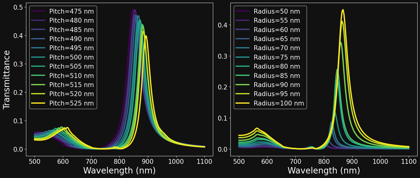
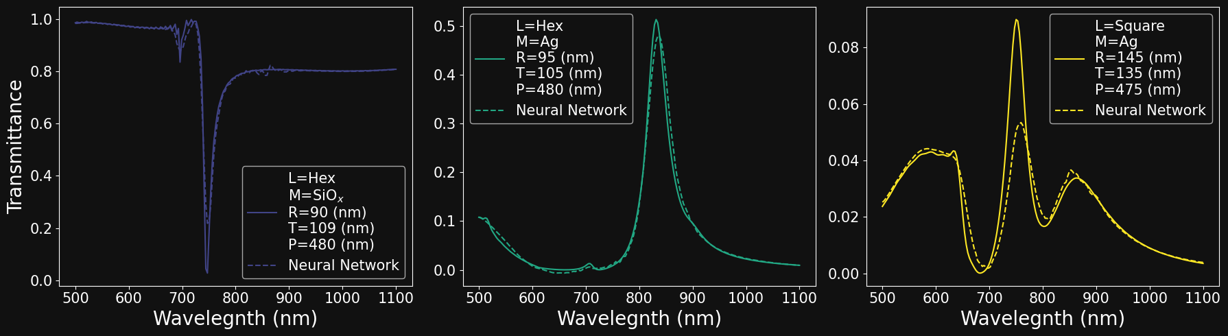
fig.set_tight_layout('tight')# Select a set of parameters
L = 0 # hexagonal lattice
M = 0 # au material
R = 100 # radius
T = 125 # thickness
P = 500 # pitch
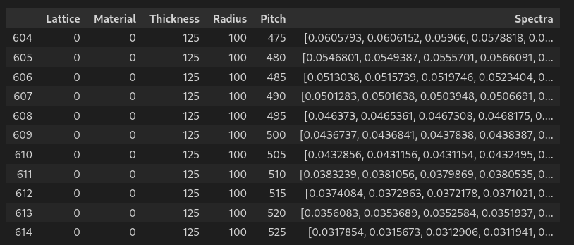
# Fix all parameters except pitch
df_pitch = df[(df.Lattice==L) & (df.Material==M) & (df.Radius==R) & (df.Thickness==T)]
df_pitch.sort_values(by=['Pitch'],inplace=True)
# Fig all parameters except radius
df_radius = df[(df.Lattice==L) & (df.Material==M) & (df.Pitch==P) & (df.Thickness==T)]
df_radius.sort_values(by=['Radius'],inplace=True)PITCH SWEEP
RADIUS SWEEP
Direct: \( g_{_{W}}:\mathbb{R}^{5} \to \mathbb{R}^{200} \)
# Importing auxiliary libraries
import numpy as np
import pandas as pd
import matplotlib.pyplot as plt
from sklearn.model_selection import train_test_split
from datetime import datetime

# import pytorch
import torch
import torch.nn as nn
from torch.utils.data import DataLoader


# import tensorboard for logging
from torch.utils.tensorboard import SummaryWriter

# importing local code
import sys
sys.path.append('../')
from datasets import SpectraDataset
from models import MLP, ResidualMLP
from loops import train,val# filename
filename = './DL-Assisted-NHA-Inverse-Design-/Dataset 6655.csv'
# load in dataframe
df = pd.read_csv(filename)
# clean and rearrange data
df['Spectra'] = df.values[:,5:][:,::-1].tolist()
df['Spectra'] = df['Spectra'].apply(np.array)
df.drop(df.columns[5:-1], axis=1, inplace=True)
df.columns = ['Lattice','Material','Thickness','Radius','Pitch','Spectra']# select and normalize input features (X)
X_df = df[['Lattice','Material','Thickness','Radius','Pitch']]
X_df = X_df/X_df.max()
# select output labels (y)
y_df = df['Spectra']
# split in training and validation set
test_val_split = 0.1 # portion of data assigned to validation set
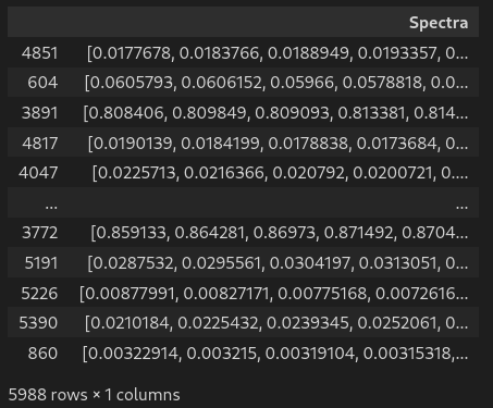
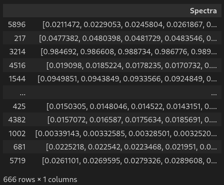
X_train, X_val, y_train, y_val = train_test_split(X_df, y_df, test_size=test_val_split, random_state=42)\( X_{train} \)
\( X_{val} \)
\( y_{train} \)
\( y_{val} \)
# import libraries
import torch
import torch.utils.data as data
import numpy as np

class SpectraDataset(data.Dataset):
    """
    Custom dataset class for loading and processing spectral data.

    Args:
        X_df (pd.DataFrame): DataFrame containing the features.
        y_df (pd.DataFrame): DataFrame containing the labels.
    """

    def __init__(self, X_df, y_df):
        """
        Initializes the dataset with the provided features and labels.
        """

        # storing dataframes as features and labels
        self.X = X_df
        self.y = y_df

    def __len__(self):
        """
        Returns the length of the dataset (number of samples).
        """

        return len(self.X)

    def __getitem__(self, idx):
        """
        Retrieves a X and y pair for a given index.
        """

         # Extract features and labels from the data
        X = torch.tensor(self.X.iloc[idx].values.astype(np.float32))
        y = torch.tensor(self.y.iloc[idx].astype(np.float32))
return X, y# instantiate training and validation dataset
training_dataset = SpectraDataset(X_train,y_train)
val_dataset = SpectraDataset(X_val,y_val)# batch size
batch_size = 64
# Create data loaders
train_dataloader = DataLoader(training_dataset, batch_size=batch_size, shuffle= True)
val_dataloader = DataLoader(val_dataset, batch_size=batch_size)
for X, y in val_dataloader:
print(f"Shape of X [N, C]: {X.shape}")
print(f"Shape of y: {y.shape} {y.dtype}")
breakShape of X [N, C]: torch.Size([64, 5])
Shape of y: torch.Size([64, 200]) torch.float32# pytorch building blocks
import torch.nn as nn
# Simple example of multilayer perceptron
class SimpleMLP(nn.Module):
def __init__(self):
super().__init__()
# first layer
self.linear1 = nn.Linear(5, 1000, bias=False)
self.activation1 = nn.ReLU()
# second layer
self.linear2 = nn.Linear(1000, 1000, bias=False)
self.activation2 = nn.ReLU()
# third layer
self.linear3 = nn.Linear(1000, 1000, bias=False)
self.activation3 = nn.ReLU()
# fourth layer
self.linear4 = nn.Linear(1000, 1000, bias=False)
self.activation4 = nn.ReLU()
# fifth layer
self.linear5 = nn.Linear(1000, 1000, bias=False)
self.activation5 = nn.ReLU()
# sixth layer
self.linear6 = nn.Linear(1000, 200, bias=False)
def forward(self, x):
# forward pass of the nn
x = self.linear1(x)
x = self.activation1(x)
x = self.linear2(x)
x = self.activation2(x)
x = self.linear3(x)
x = self.activation3(x)
x = self.linear4(x)
x = self.activation4(x)
x = self.linear4(x)
x = self.activation4(x)
x = self.linear5(x)
x = self.activation5(x)
x = self.linear6(x)
return x# 1pytorch building blocks
import torch.nn as nn
# a flexible, fully connected base block
class BaseBlock(nn.Module):
def __init__(self, in_features, out_features, p=0.2, activation=nn.GELU()):
super().__init__()
self.linear = nn.Linear(in_features, out_features, bias=False)
self.dropout = nn.Dropout(p=p)
self.activation = activation
def forward(self, x):
x = self.linear(x)
x = self.activation(x)
x = self.dropout(x)
return x
# a simple linear block for the direct regression problem
class LinearBlock(nn.Module):
def __init__(self, in_features, out_features):
super().__init__()
self.linear = nn.Linear(in_features, out_features, bias=False)
def forward(self, x):
x = self.linear(x)
return x# pytorch building blocks
import torch.nn as nn
from layers import BaseBlock, LinearBlock
# A flexible implementation of the multilayer perceptron
class FlexibleMLP(nn.Module):
def __init__(
self,
hidden_layers=[5, 1000, 1000, 1000, 1000, 1000, 200],
p=0.2,
activation=nn.GELU(),
):
super().__init__()
self.layers = nn.ModuleList()
for i in range(1, len(hidden_layers) - 1):
self.layers.append(
BaseBlock(
hidden_layers[i - 1], hidden_layers[i], p=p, activation=activation
)
)
self.final_block = LinearBlock(hidden_layers[-2], hidden_layers[-1])
def forward(self, x):
for layer in self.layers:
x = layer(x)
x = self.final_block(x)
return x# Get cpu or gpu device for training.
device = (
"cuda"
if torch.cuda.is_available()
else "cpu"
)
print(f"Using {device} device")# base learning rate
lr = 1.1e-4
# defining loss and optimizer
loss_fn = nn.MSELoss()
optimizer = torch.optim.Adam(model.parameters(),lr=lr)# the training loop
def train(dataloader, model, loss_fn, optimizer, device):
size = len(dataloader.dataset)
model.train()
for batch, (X, y) in enumerate(dataloader):
X, y = X.to(device), y.to(device)
# Compute prediction error
pred = model(X)
loss = loss_fn(pred, y)
# Backpropagation
loss.backward()
optimizer.step()
optimizer.zero_grad()
if batch % 100 == 0:
loss, current = loss.item(), (batch + 1) * len(X)
print(f"Train loss: {loss:>7f} [{current:>5d}/{size:>5d}]")
return loss# the validation loop
def val(dataloader, model, loss_fn, device):
num_batches = len(dataloader)
model.eval()
val_loss = 0
with torch.no_grad():
for X, y in dataloader:
X, y = X.to(device), y.to(device)
pred = model(X)
val_loss += loss_fn(pred, y).item()
val_loss /= num_batches
print("\n")
print(f"Validation loss: {val_loss:>8f} \n")
return val_loss# create timestamp
now = datetime.now() # current date and time
date_time = now.strftime("%d%m%y_%H%M%S")
# create summary writer for tensorboard
writer_path = '../tb_logs/' + date_time + '/'
writer = SummaryWriter(writer_path)
# loop over epochs
epochs = 2500
epoch_threshold = 500
save_checkpoint = './best_model_' + date_time + '.ckpt'
best_loss = 1.0
for epoch in range(epochs):
# log epoch to console
print(f"Epoch {epoch+1}\n-------------------------------")
# performe training and validation loops
train_loss = train(train_dataloader, model, loss_fn, optimizer, device)
val_loss = val(val_dataloader, model, loss_fn, device)
# log training and validation loss to console
writer.add_scalar("Loss/train", train_loss, epoch)
writer.add_scalar("Loss/val", val_loss, epoch)
# save checkpoint
if (val_loss < best_loss) and (epoch>epoch_threshold):
# save checkpoint
model.train()
torch.save(model.state_dict(), save_checkpoint)
best_loss = val_loss
# close connection to tensorboard
writer.flush()
writer.close()
# finished
print("Done!")# Instantiate inference model and set to evaluation mode
model_inference = FlexibleMLP(hidden_layers=hidden_layers, activation=nn.GELU(), p=0.1).to(
device)
model_inference.load_state_dict(torch.load(save_checkpoint,weights_only=True))
model_inference.eval()
# compute inference on all validation samples
X_inference = torch.tensor(X_val.to_numpy().astype(np.float32)).to(device)
y_inference = model_inference(X_inference)
y_true = torch.tensor(np.stack(y_val.to_numpy()).astype(np.float32)).to(device)
# compute normalized loss for each sample in the validation dataset
loss_fn_inference = nn.MSELoss(reduction='none')
with torch.no_grad():
loss_inference = loss_fn_inference(y_inference,y_true).sum(axis=-1)
norm_mse_discrepancy = loss_inference/((y_true**2).sum(axis=-1))
k_best = torch.argsort(norm_mse_discrepancy)# 1pytorch building blocks
import torch.nn as nn
# a flexible, fully connected, multi headed network
class FlexibleInverseMLP(nn.Module):
def __init__(
self,
hidden_layers=[200, 1000, 1000, 1000, 1000, 1000, 2, 3, 3],
p=0.2,
activation=nn.GELU(),
):
super().__init__()
self.layers = nn.ModuleList()
for i in range(1, len(hidden_layers) - 3):
self.layers.append(
BaseBlock(
hidden_layers[i - 1], hidden_layers[i], p=p, activation=activation
)
)
# define 2 classification heads and 1 regression head
self.lattice_head = LinearBlock(hidden_layers[-4], hidden_layers[-3])
self.material_head = LinearBlock(hidden_layers[-4], hidden_layers[-2])
self.geometry_head = LinearBlock(hidden_layers[-4], hidden_layers[-1])
def forward(self, x):
# common path
for layer in self.layers:
x = layer(x)
# three heads
x_lattice = self.lattice_head(x)
x_material = self.material_head(x)
x_geometry = self.geometry_head(x)
return x_lattice,x_material,x_geometry# the inverse training loop
def train_inverse(dataloader, model, loss_reg, loss_ce, optimizer, device):
size = len(dataloader.dataset)
model.train()
for batch, (X, y) in enumerate(dataloader):
X, y = X.to(device), y.to(device)
# Compute prediction error
pred_l, pred_m, pred_g = model(X)
true_l = y[:,0].type(torch.LongTensor).to(device)
true_m = y[:,1].type(torch.LongTensor).to(device)
true_g = y[:,2:].to(device)
loss = loss_ce(pred_l, true_l) + loss_ce(pred_m, true_m) + 5.0*loss_reg(pred_g, true_g)
# Backpropagation
loss.backward()
optimizer.step()
optimizer.zero_grad()
if batch % 20 == 0:
loss, current = loss.item(), (batch + 1) * len(X)
print(f"Train loss: {loss:>7f} [{current:>5d}/{size:>5d}]")
return loss# the inverse validation loop
def val_inverse(dataloader, model, loss_reg, loss_ce, device):
num_batches = len(dataloader)
model.eval()
val_loss = 0
with torch.no_grad():
for X, y in dataloader:
X, y = X.to(device), y.to(device)
pred_l, pred_m, pred_g = model(X)
true_l = y[:,0].type(torch.LongTensor).to(device)
true_m = y[:,1].type(torch.LongTensor).to(device)
true_g = y[:,2:].to(device)
loss = loss_ce(pred_l, true_l) + loss_ce(pred_m, true_m) + loss_reg(pred_g, true_g)
val_loss += loss.item()
val_loss /= num_batches
print("\n")
print(f"Validation loss: {val_loss:>8f} \n")
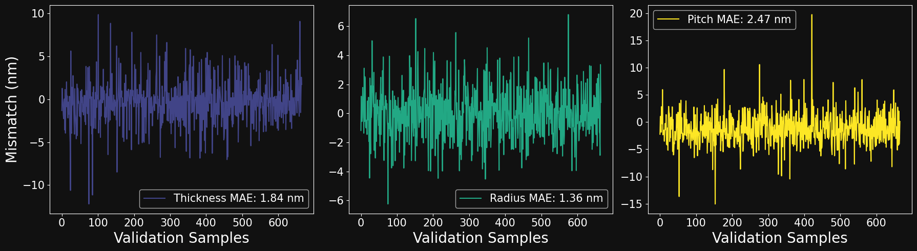
return val_loss# Instantiate inference model and set to evaluation mode
model_inference = FlexibleInverseMLP(hidden_layers=hidden_layers, activation=nn.GELU(), p=0.1).to(
device)
model_inference.load_state_dict(torch.load(save_checkpoint,weights_only=True))
model_inference.eval()
# compute inference on all validation samples
X_inference = torch.tensor(np.stack(X_val.to_numpy()).astype(np.float32)).to(device)
y_inf_lattice, y_inf_material, y_inf_geometry = model_inference(X_inference)
y_true = torch.tensor(y_val.to_numpy().astype(np.float32)).to(device)
# formatting true values for each classification and regression task
y_true_lattice = y_true[:, 0].type(torch.LongTensor).detach().cpu()
y_true_material = y_true[:, 1].type(torch.LongTensor).detach().cpu()
y_true_geometry = (
torch.stack((y_true[:, 2] * t_max, y_true[:, 3] * r_max, y_true[:, 4] * p_max))
.T.detach()
.cpu()
)
# formatting predicted values for each classification and regression task
y_pred_lattice = (
torch.argmax(torch.nn.functional.softmax(y_inf_lattice, dim=-1), dim=-1)
.detach()
.cpu()
)
y_pred_material = (
torch.argmax(torch.nn.functional.softmax(y_inf_material, dim=-1), dim=-1)
.detach()
.cpu()
)
y_pred_geometry = (
torch.stack(
(
y_inf_geometry[:, 0] * t_max,
y_inf_geometry[:, 1] * r_max,
y_inf_geometry[:, 2] * p_max,
)
)
.T.detach()
.cpu()
)