Monosynaptic Scalable Architecture Revealed by Transsynaptic Rabies Tracing
Daniel Fürth
Meletis Lab
Network for Networks
12 Feb 2016
daniel.furth@ki.se
- Yang Xuan
- Ourania Tzortzi
- Iakovos Lazardis
- Konstantinos Meletis
- DMC lab
Acknowledgement
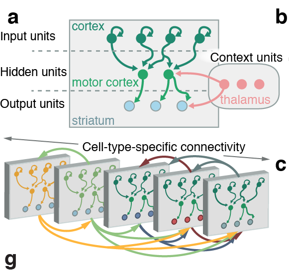
Reconstructing brain from sectioned tissue
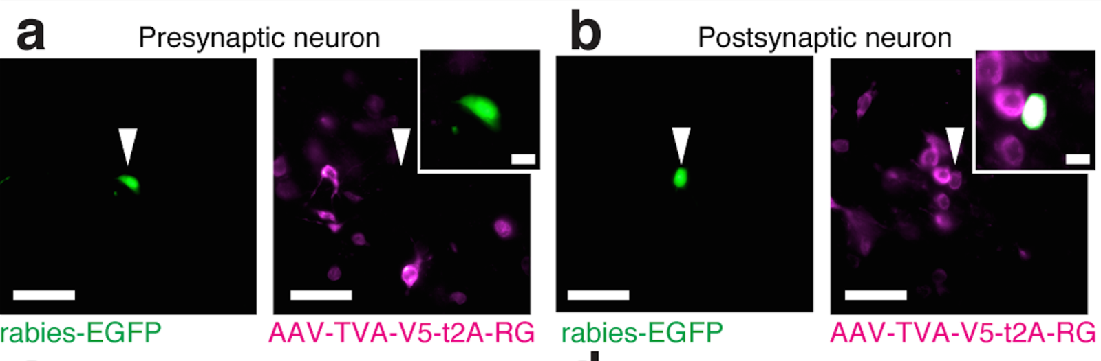
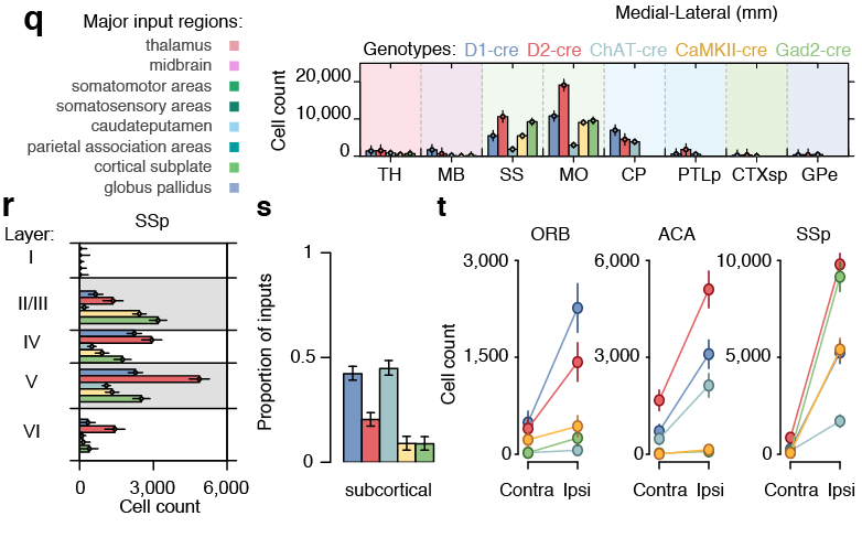
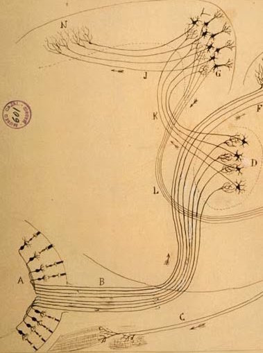
Tracing the network
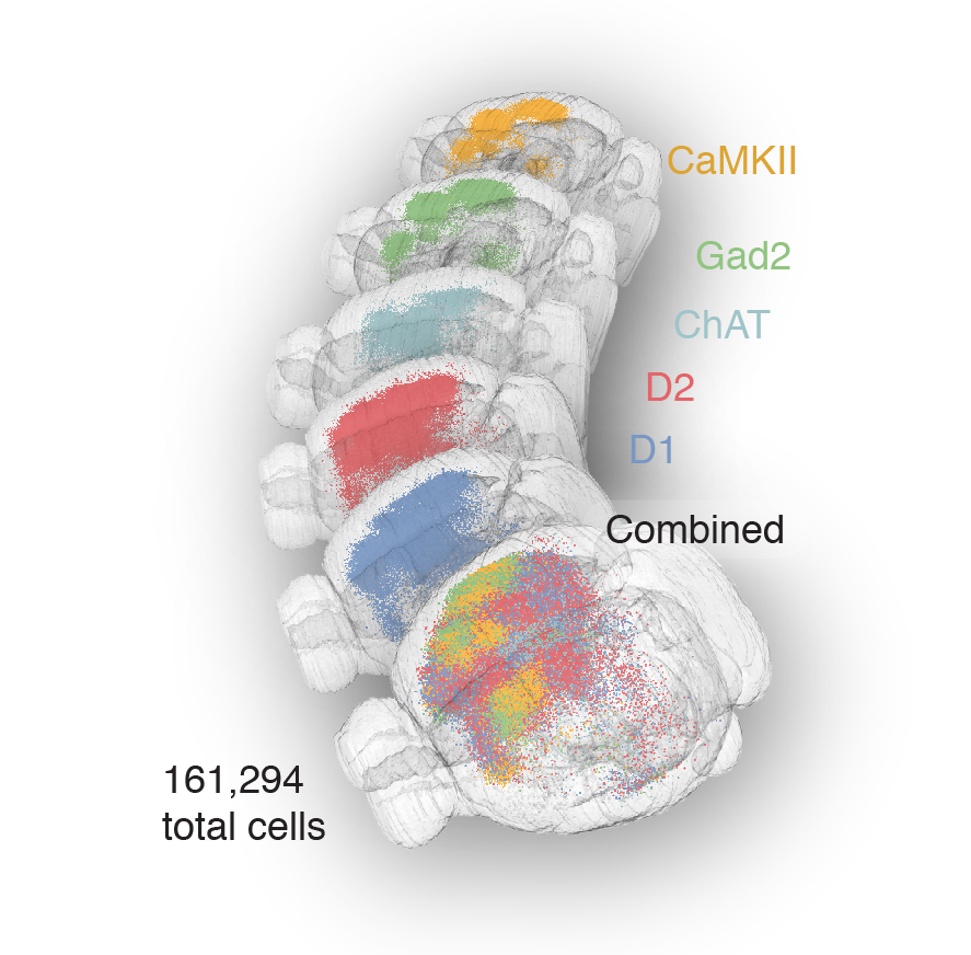
Tracing the network
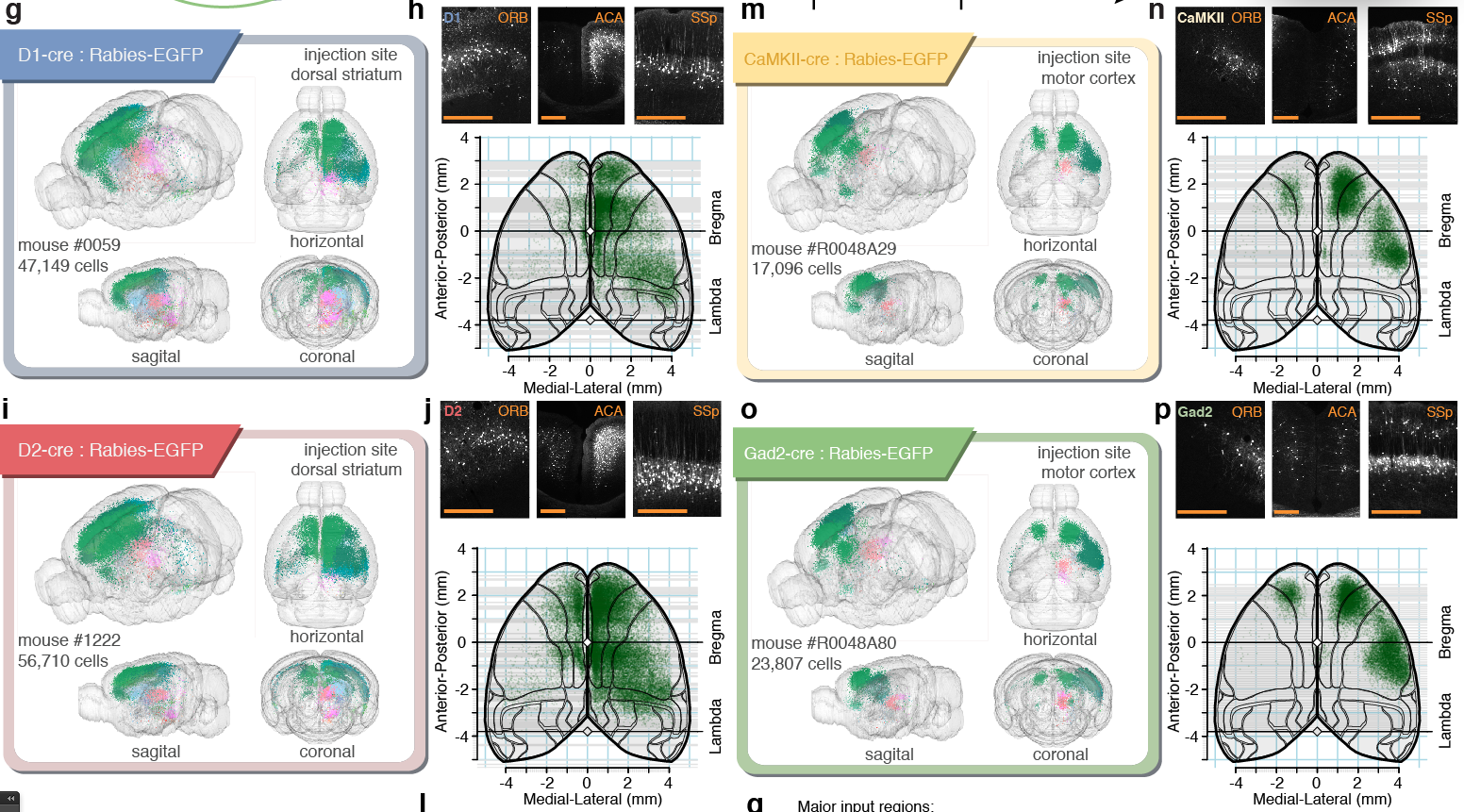
Tracing the network
Scaling rules for rodent brians
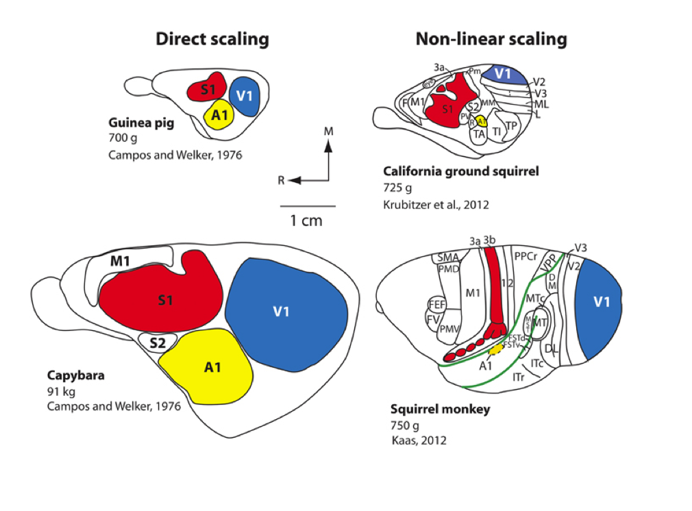
Isometric
Allometric
Cellular scaling rules for rodent brians

Herculano-Houzel et al. PNAS
Cellular scaling rules
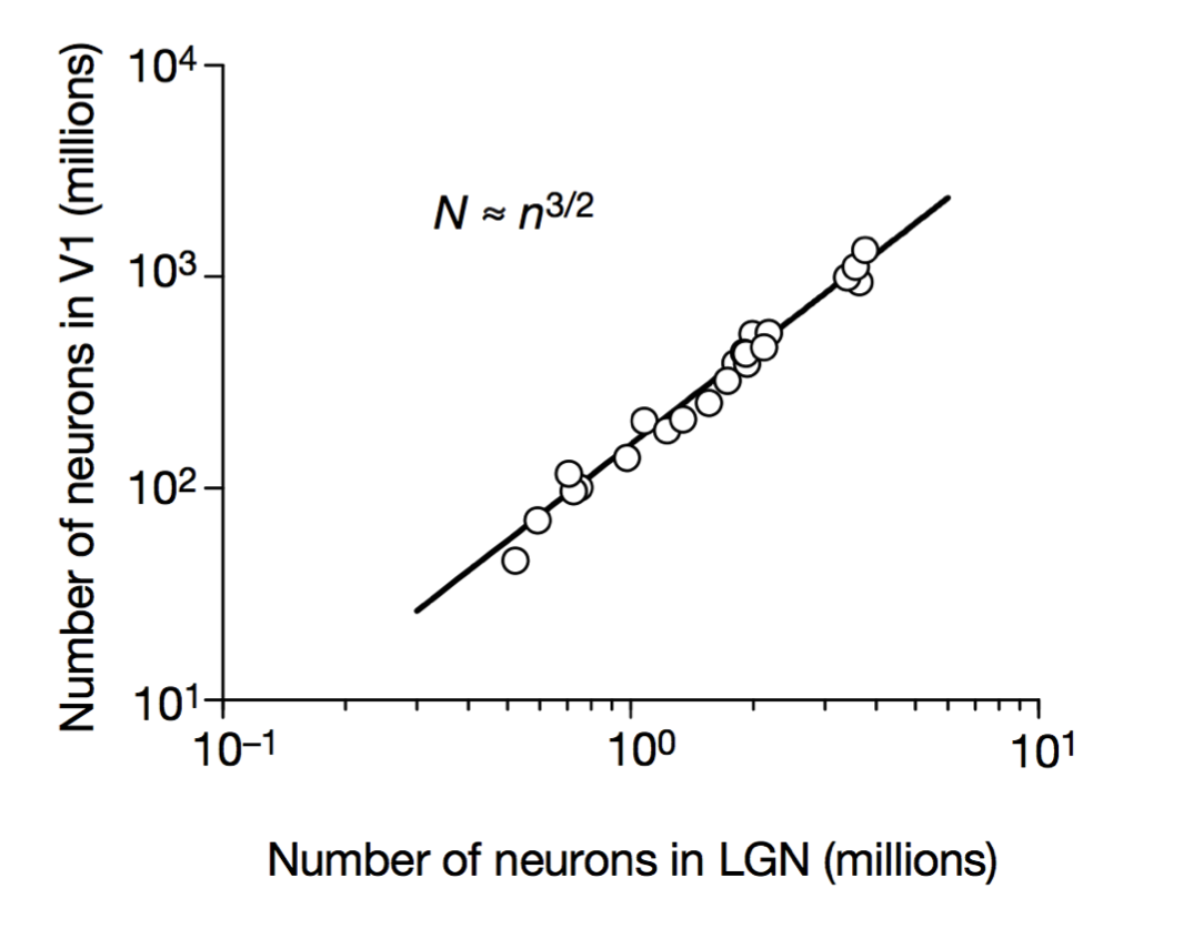
Stevens (2000) Nature
Cellular scaling rules
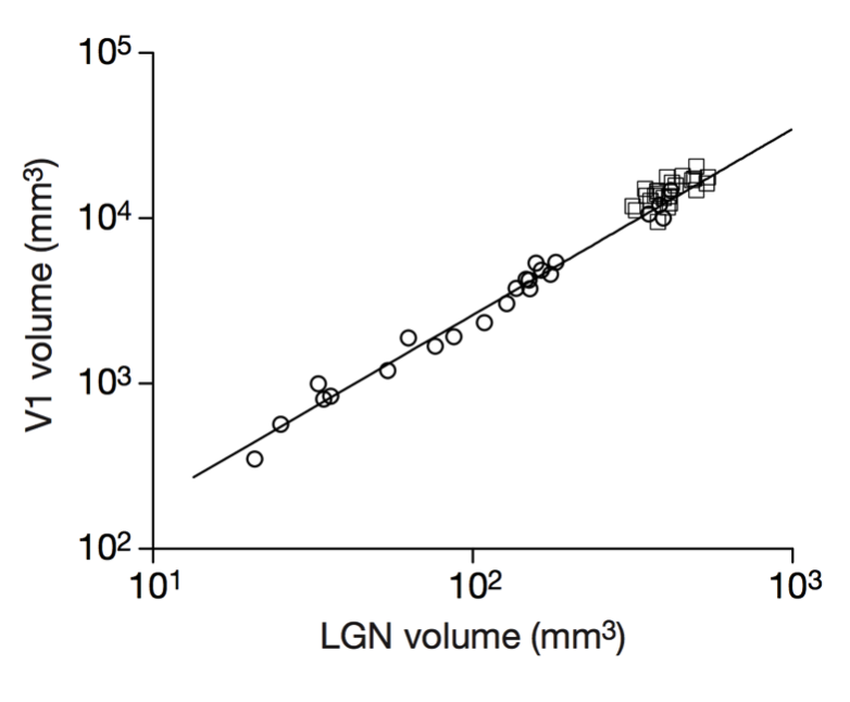
Stevens (2000) Nature
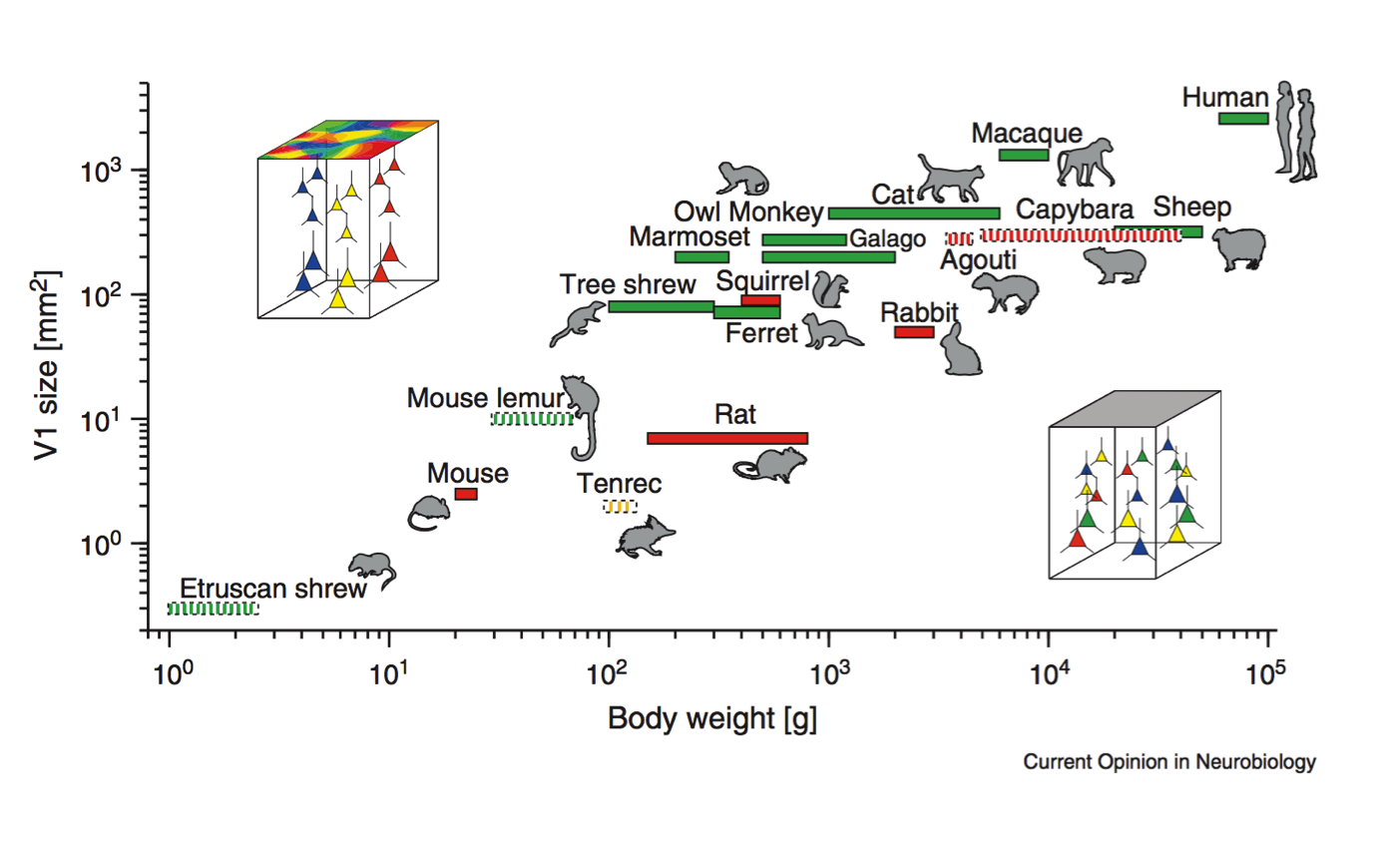
Cellular scaling rules
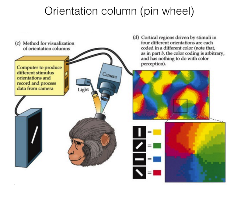
Hubel & Wiesel (1974), Blasdel (1986)
Cellular scaling rules

Cellular scaling rules
Stevens (2000) Nature
Cellular scaling rules
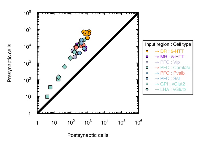
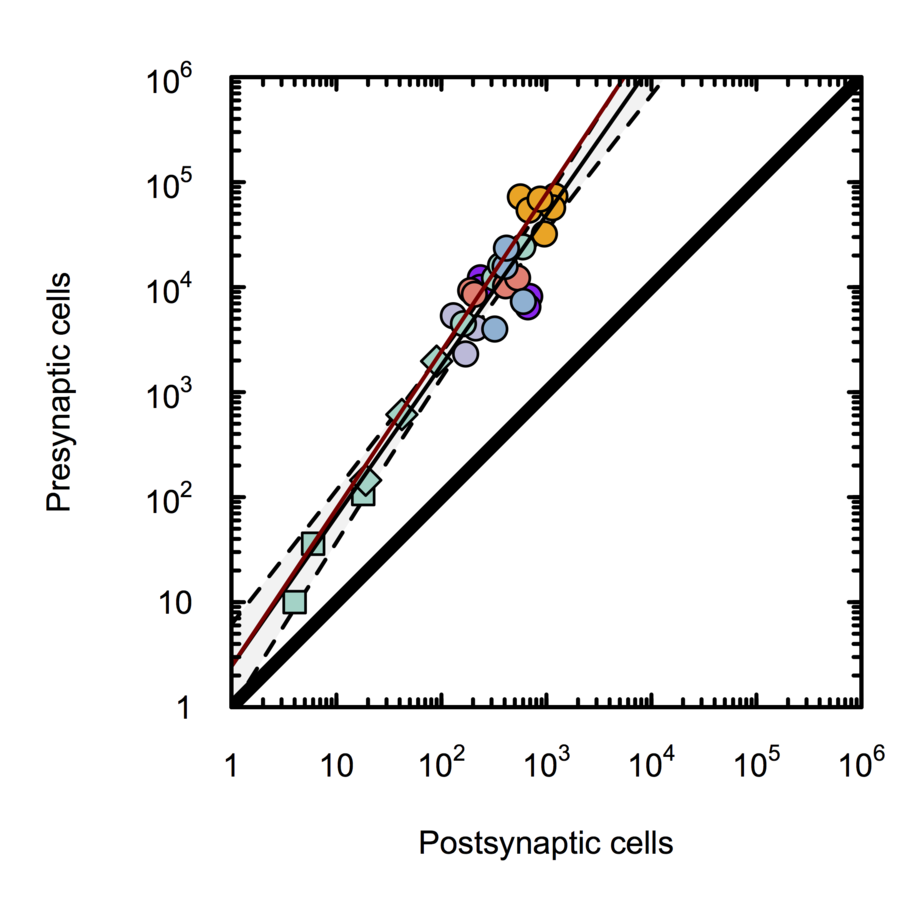
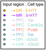
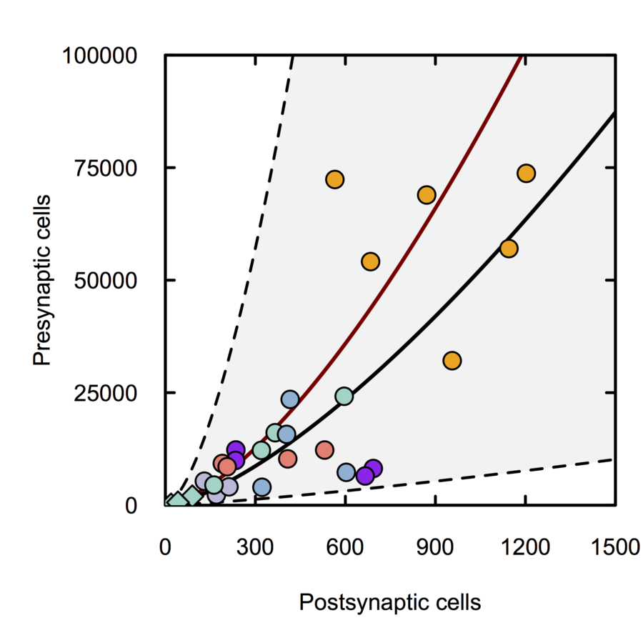
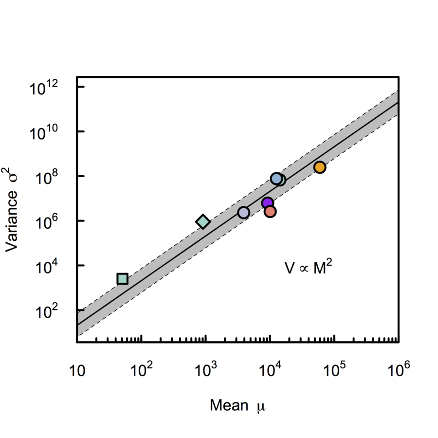
Monosynaptic scaling in mice
Synapse density and dendritic branching
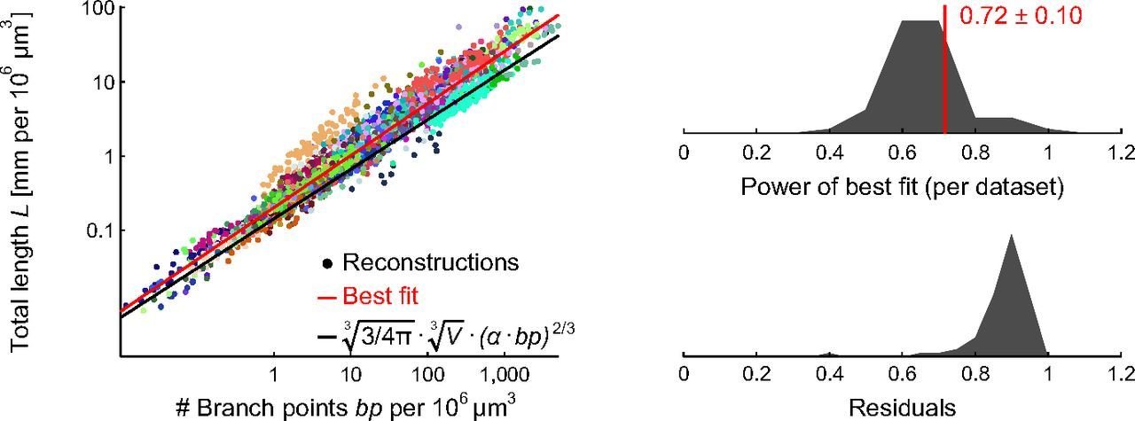
Cuntz, Mathy & Häusser (2012) PNAS
Synapse density and dendritic branching
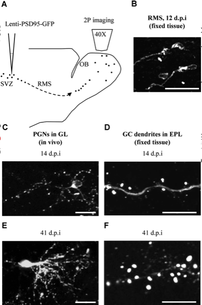
Livneh, Feinstein, Klein and Mizrahi (2009) JoN
Synapse density and dendritic branching
Cuntz, Mathy & Häusser (2012) PNAS

Synapse density and dendritic branching
Cuntz, Mathy & Häusser (2012) PNAS
Self-organizing branching process
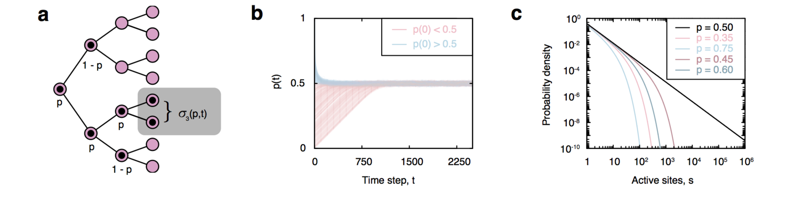
Self-organizing branching process
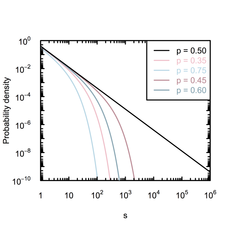
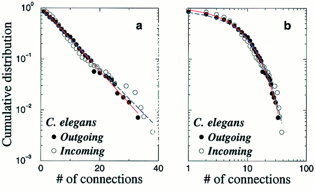
Amaral et al. (2000); White, Southgate, Thompson & Brenner (1986)
Mean-field results
Total output for the network:
Total connection of type k for ith neuron:
Average number of connections in network
Mean-field results
Cost per unit length for dendrite to cover an area
Set average number of connections to the cost for the dendritic tree
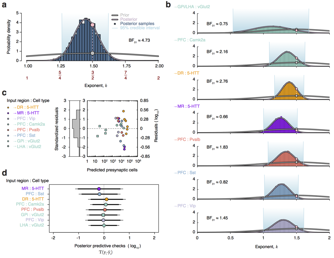
Bayesian inference
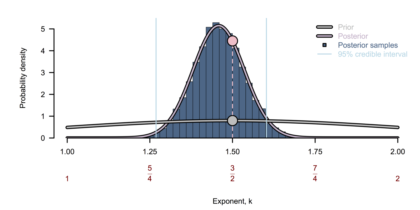
Bayesian inference
Dendritic pruning as an age-dependent branching process
Cowan, (1984), Azevedo & Leroi (2000) PNAS


Data you shouldn't
go to war on
Data you do
go to war on
Thank you!
scRNA-seq
Gene specificity
about ~24'000 genes expressed in the brain.