Mapping single-cell RNA sequencing (scRNAseq) data to tissue of origin using in situ hybridization
Daniel Fürth
Meletis Lab
ISH course
11th March 2016
daniel.furth@ki.se
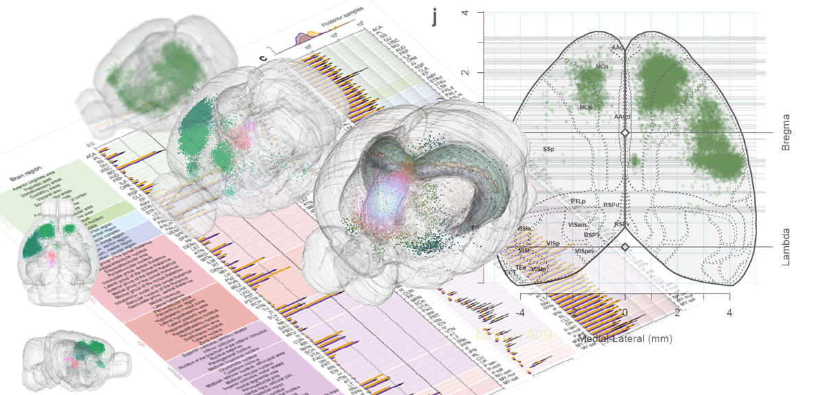
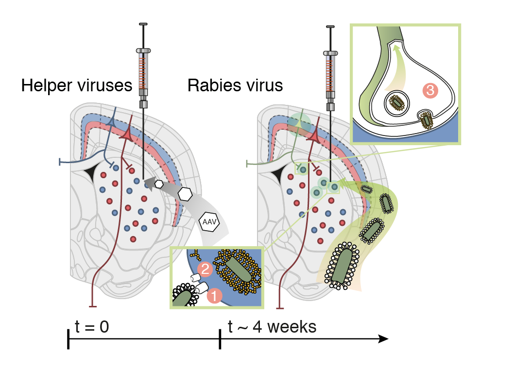
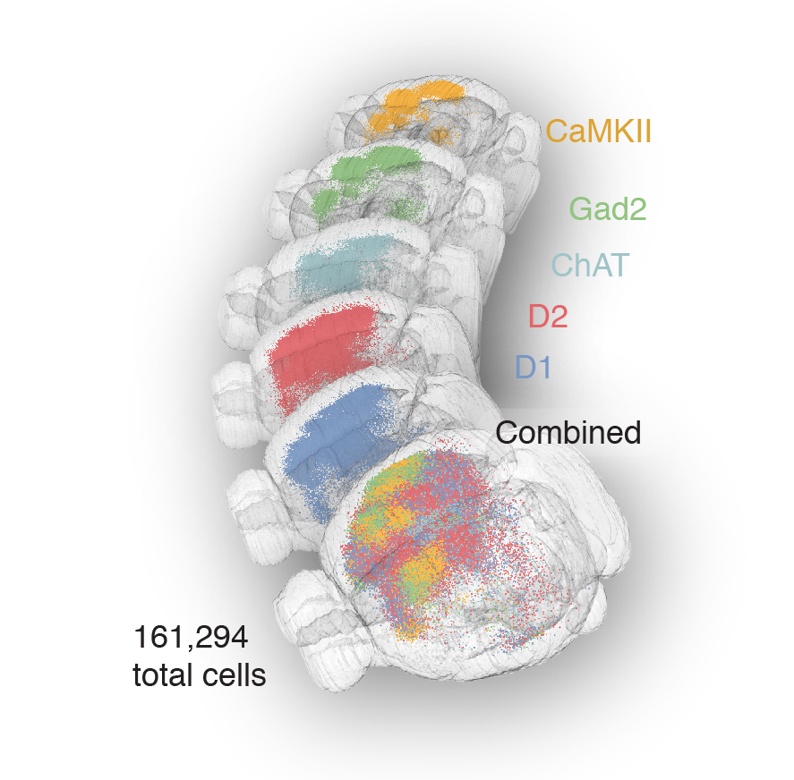
Tracing the network
Tracing the network
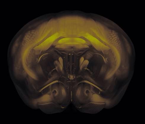
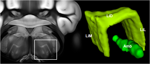
Whole-Brain Reconstruction
Pollak Dorocic et al. 2014


Reconstructing brain from sectioned tissue
Tracing the network
DRD2 film
56,710 neurons
Tracing the network
Tracing the network
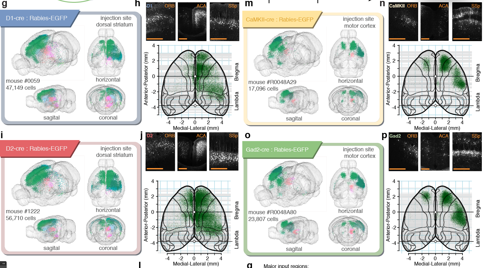
Tracing the network
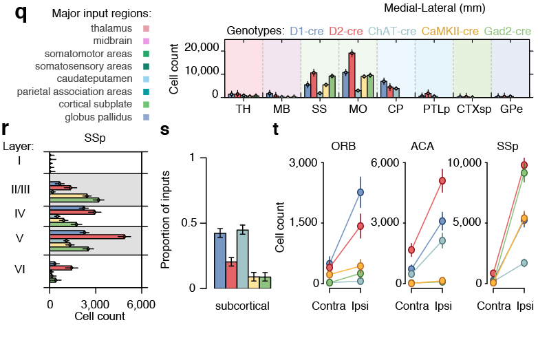
'Google maps' of neuroanatomy
'Google maps' of neuroanatomy


similar to...
works with...
scRNA-seq
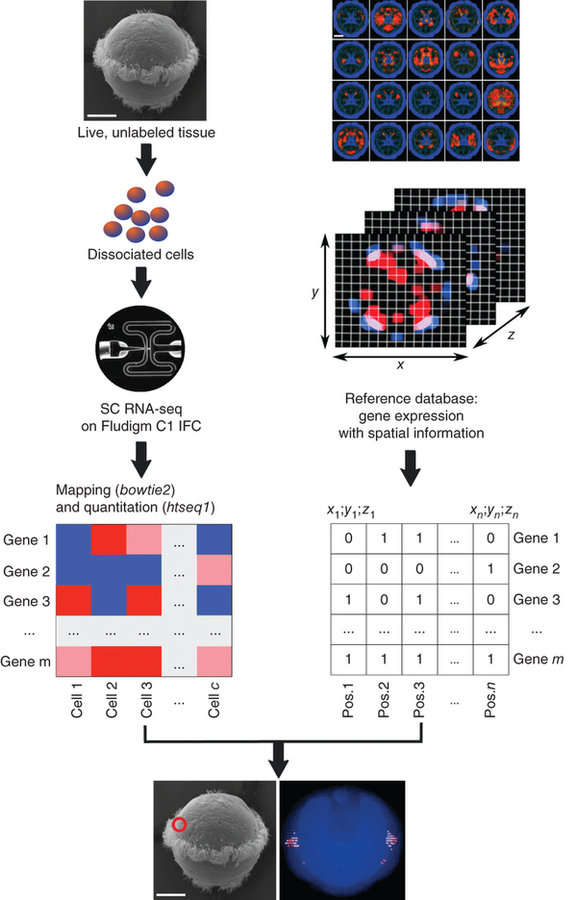
NATURE BIOTECHNOLOGY | COMPUTATIONAL BIOLOGY | ANALYSIS
High-throughput spatial mapping of single-cell RNA-seq data to tissue of origin
Kaia Achim, Jean-Baptiste Pettit, Luis R Saraiva, Daria Gavriouchkina, Tomas Larsson, Detlev Arendt & John C Marioni
scRNA-seq
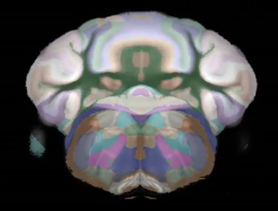
Allen Brain Reference Atlas

-
Atlas 2007 (manually drawn Nissl):
- 200 μm thick coronal sections.
-
Atlas 2011:
- 100 μm both coronal and sagital
- Atlas 2014 (connectivity avrg template)
-
Atlas 2015 (beginning of june):
- 10 x 50 μm
-
Registration atlas:
- 25 x 25 μm
-
Grid expression ISH:
- 200 x 200 μm MetaIOimage (.raw, .mhd)
scRNA-seq
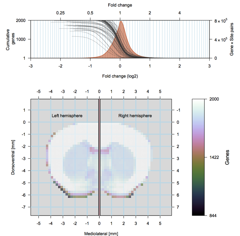
Anatomic Gene Expression Atlas
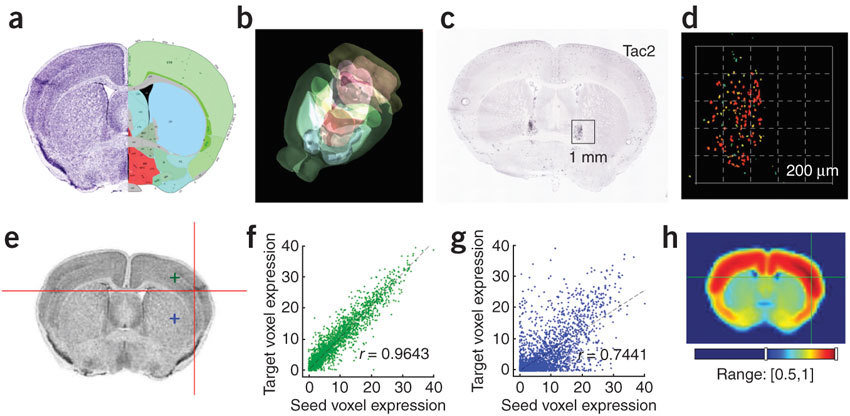
Lydia Ng, et al. (2009) Nat. Neuro.
http://mouse.brain-map.org/agea
scRNA-seq
scRNA-seq
Allen Brain Reference Atlas
scRNA-seq
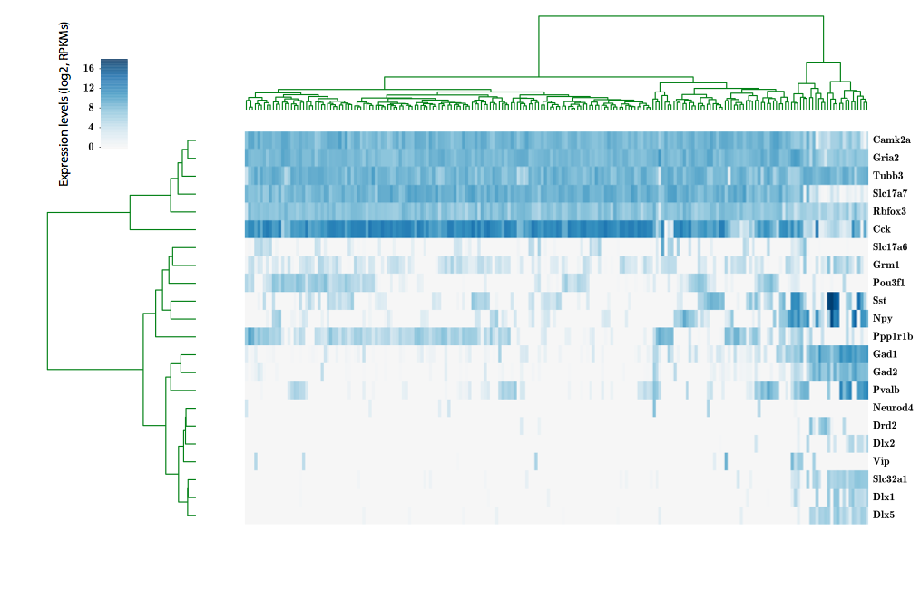
324 cells from cortico-striatal section
scRNA-seq
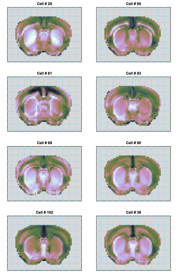
Our approach
scRNA-seq
Our approach
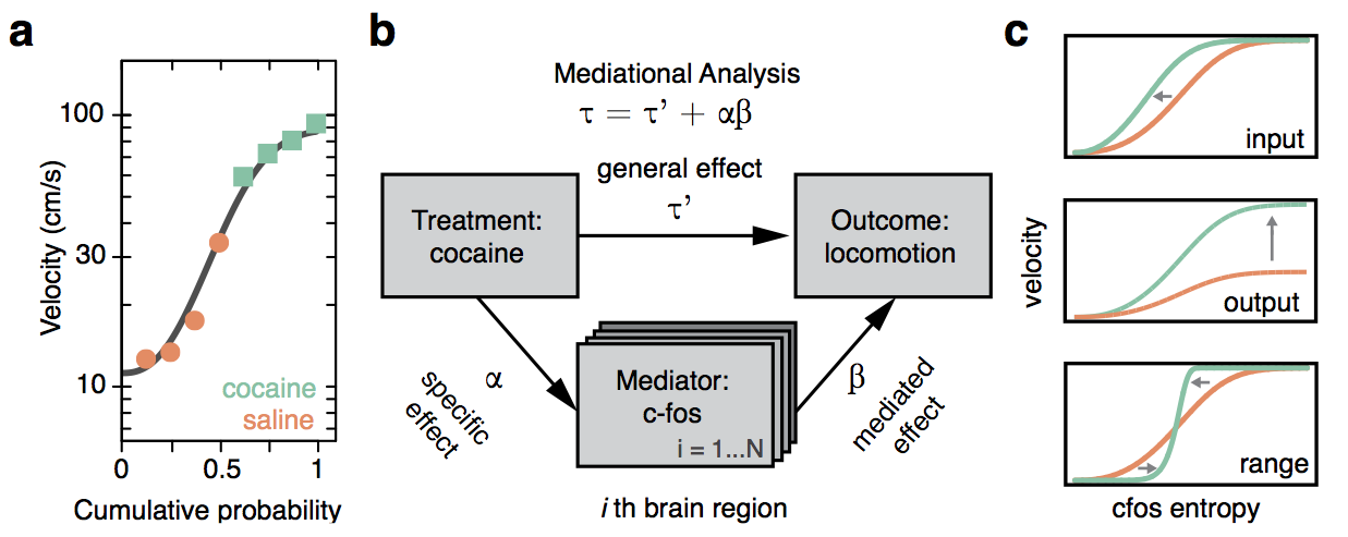
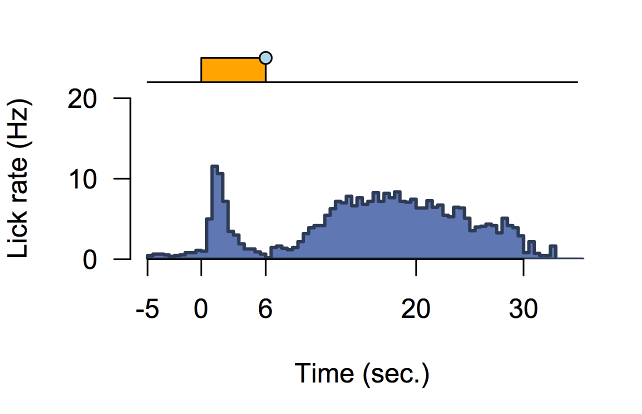
understanding behavior
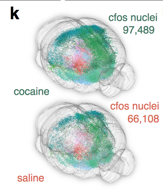
Cocaine induced locomotoric activity
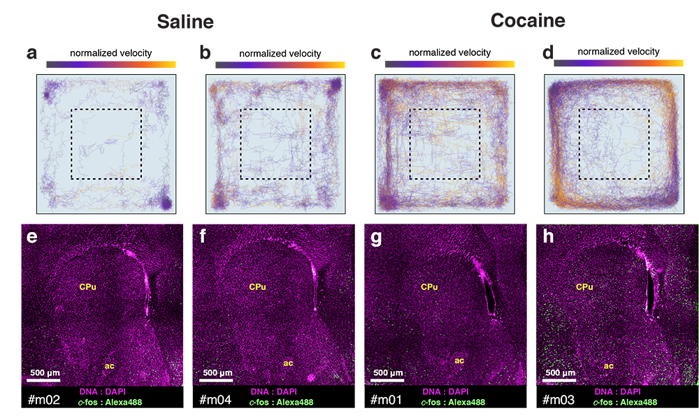
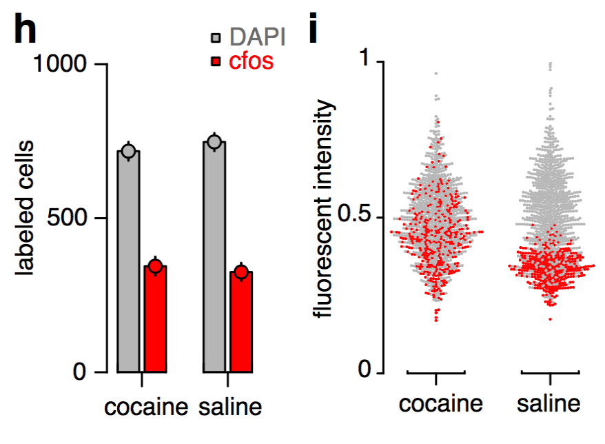
Whole-brain behavioral c-Fos mapping
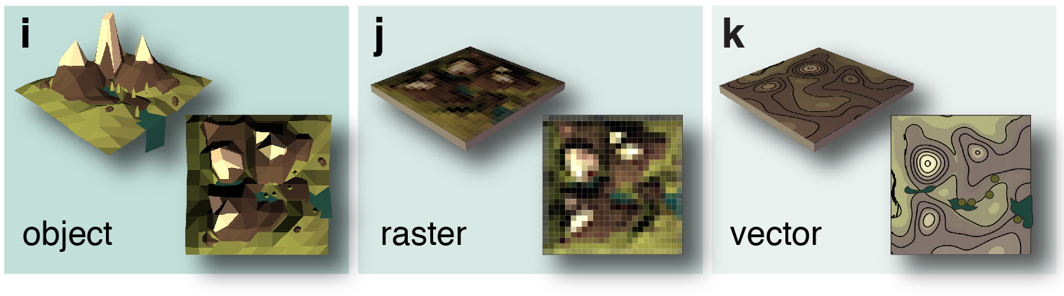
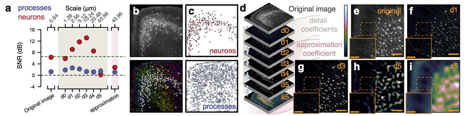
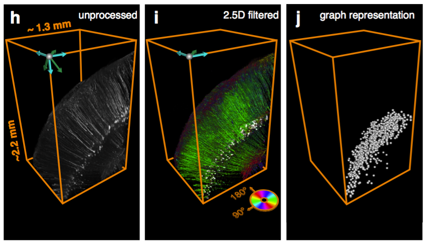
Multiresolution decomposition
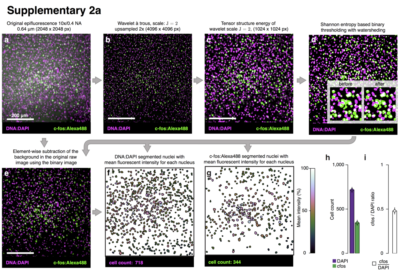
Multiresolution decomposition
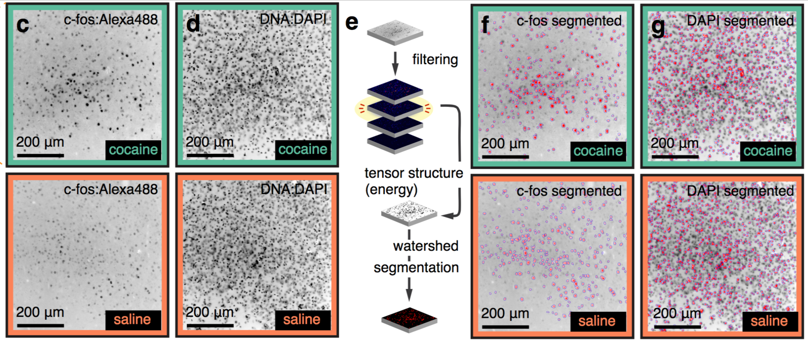
Multiresolution decomposition
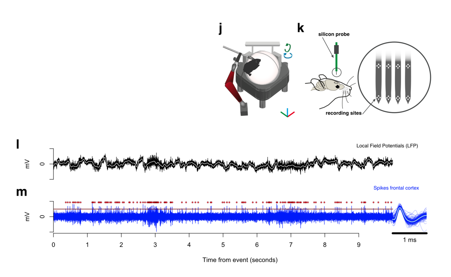
Fluorescent microscope technologies
Multiplexed Intact-Tissue Transcriptional Analysis at Cellular Resolution. Cell 2016

Fluorescent microscope technologies
Multiplexed Intact-Tissue Transcriptional Analysis at Cellular Resolution. Cell 2016
Fluorescent microscope technologies
Multiplexed Intact-Tissue Transcriptional Analysis at Cellular Resolution. Cell 2016
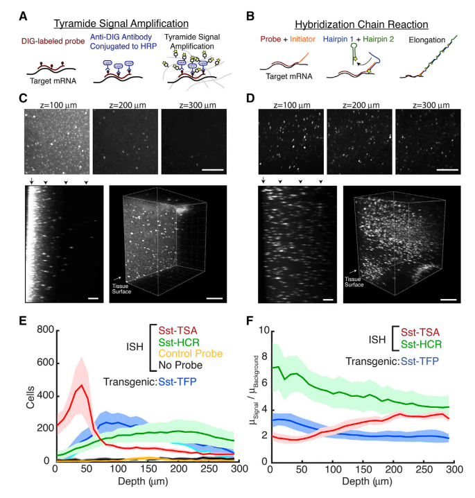
Comparison of Antibody-Based and DNA-Based Amplification
Multiresolution decomposition
Fluorescent microscope technologies
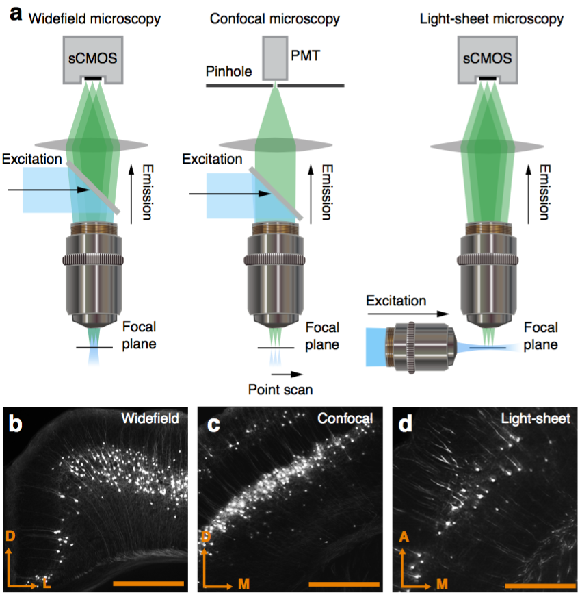
Fluorescent microscope technologies
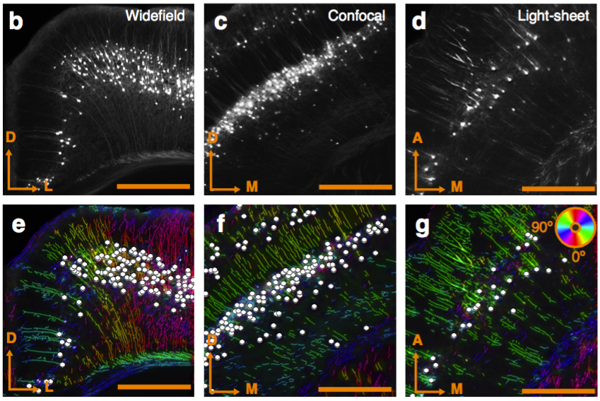
Fluorescent microscope technologies
scRNA-seq
Allen Brain Reference Atlas

-
Atlas 2007 (manually drawn Nissl):
- 200 μm thick coronal sections.
-
Atlas 2011:
- 100 μm both coronal and sagital
- Atlas 2014 (connectivity avrg template)
-
Atlas 2015 (beginning of june):
- 10 x 50 μm
-
Registration atlas:
- 25 x 25 μm
-
Grid expression ISH:
- 200 x 200 μm MetaIOimage (.raw, .mhd)
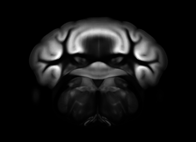
Connectivity average template (Ng et al. 2014)
scRNA-seq
Allen Brain Reference Atlas
-
Atlas 2007 (manually drawn Nissl):
- 200 μm thick coronal sections.
-
Atlas 2011:
- 100 μm both coronal and sagital
- Atlas 2014 (connectivity avrg template)
-
Atlas 2015 (beginning of june):
- 10 x 50 μm
-
Registration atlas:
- 25 x 25 μm
-
Grid expression ISH:
- 200 x 200 μm MetaIOimage (.raw, .mhd)
Connectivity average template (Ng et al. 2014)
Functional
Can be used to segment processes and their direction.
CLARITY
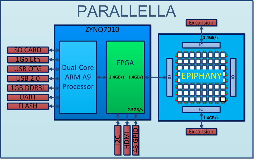
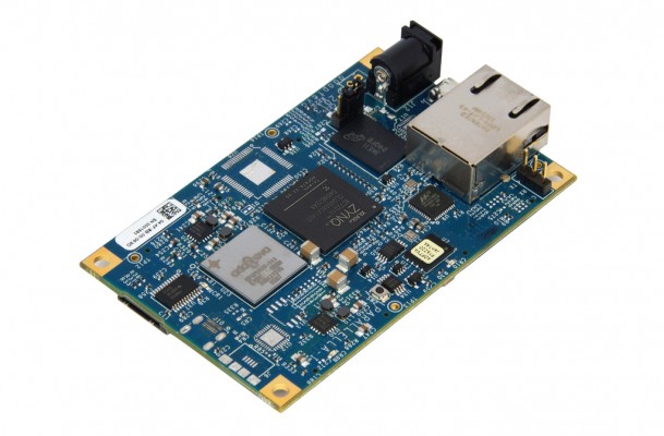
Do we really have a 'BigData' problem in neuroscience?

http://www.parallac.org/
10 computers (146 processors)
Up to 64 cores per processor!
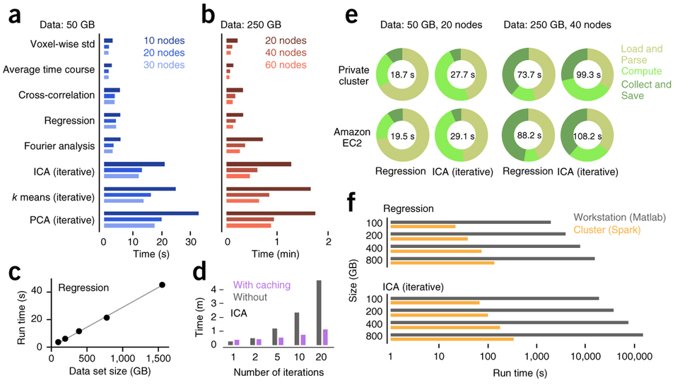
Freeman et al. (2014) Nature Methods
R package
- Why R?
- Standard data analysis:
- load some data
- estimate the density distribution.
- plot it
- Standard data analysis:
xx <- faithful$eruptions
fit <- density(xx)
plot(fit)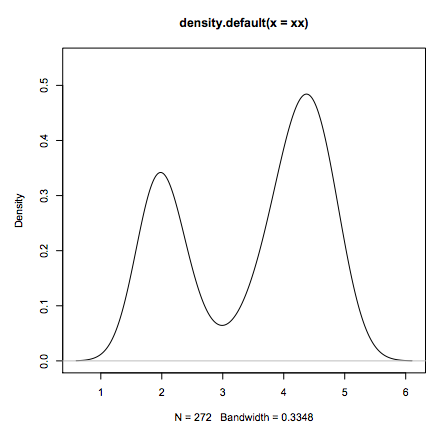
R package
- Why R?
#Line 1: loading
xx <- faithful$eruptions
#Line 2: estimate density
fit1 <- density(xx)
#Line 2: draw 10'000 bootstraps
fit2 <- replicate(10000, {
    x <- sample(xx,replace=TRUE);
    density(x, from=min(fit1$x), to=max(fit1$x))$y
})
#Line 3: compute 95% error "bars"
fit3 <- apply(fit2, 1, quantile,c(0.025,0.975))
#Line 4: plot the estimate
plot(fit1, ylim=range(fit3))
#Line 5: add estimation error as shaded region
polygon(c(fit1$x,rev(fit1$x)), c(fit3[1,], rev(fit3[2,])), col=’grey’, border=F)
#Line 6: add the line again since the polygon overshadows it.
lines(fit1)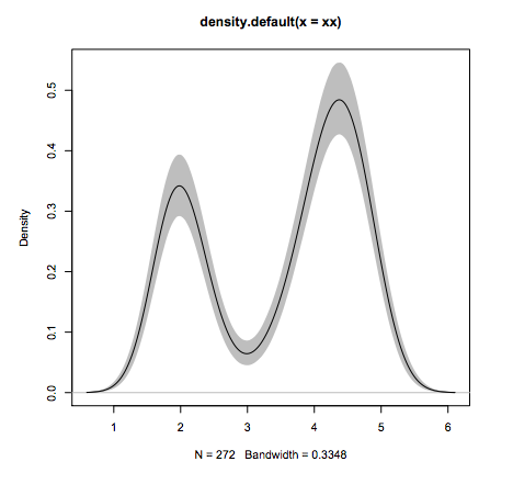
What other language can do this in 6 lines of code?
Parallel computing
- Parallel computing is extremely simple to implement from R.
# install.packages('foreach'); install.packages('doSNOW')
library(foreach)
library(doSNOW)
cl <- makeCluster(2, type = "SOCK")
registerDoSNOW(cl)

getDoParName()


#matrix operators
x <- foreach(i=1:8, .combine='rbind', .packages='wholebrain' ) %:%
   foreach(j=1:2, .combine='c', .packages='wholebrain' ) %dopar% {
     l <- runif(1, i, 100)
     i + j + l
   }
Concurrency and parallel programming
- Multi threaded applications through .

#include <string>
#include <iostream>
#include <thread>

using namespace std;

//The functions we want to make the thread run.
void task1(string msg)
{
    cout << "task1 says: " << msg;
}

void task2(string msg)
{
    cout << "task1 says: " << msg;
}

//Main loop.
int main()
{
    thread t1(task1, "Task 1 executed");
    thread t2(task2, "Task 1 executed");
    t1.join();
    t2.join();
}
Rcpp
Concurrency and parallel programming
- Multi-threaded applications through .
#include <string>
#include <iostream>
#include <thread>

using namespace std;

//The functions we want to make the thread run.
void task1(string msg)
{
    cout << "task1 says: " << msg;
}

void task2(string msg)
{
    cout << "task1 says: " << msg;
}

//Main loop.
int main()
{
    thread t1(task1, "Task 1 executed");
    thread t2(task2, "Task 1 executed");
    //let main wait for t1 and t2 to finish.
    t1.join();
    t2.join();
}
Rcpp
Dual core
Thank you!
scRNA-seq
Gene specificity
about ~24'000 genes expressed in the brain.