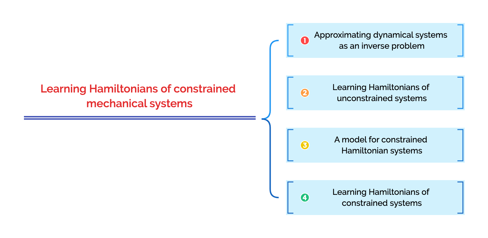
Learning Hamiltonians of constrained systems

Learning Hamiltonians of constrained mechanical systems

Davide Murari

Machine Learning and Dynamical Systems

Alan Turing Institute - 05/05/2022

\(\texttt{davide.murari@ntnu.no}\)

Joint work with Elena Celledoni, Andrea Leone and Brynjulf Owren

Definition of the problem

\dot{x}(t) = f(x(t))\in\mathbb{R}^m

GOAL : approximate the unknown \(f\) on \(\Omega\)

DATA:

\{(x_i,y_i^1,...,y_i^M)\}_{i=1,...,N},\\ x_i\in\Omega\subset\mathbb{R}^m

y_i^j = \Phi_f^{j\Delta t}(x_i) + \delta_i^j

\Delta t>0

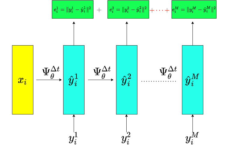
Approximation of a dynamical system

Introduce a parametric model

\dot{x}(t) = \hat{f}_{\theta}(x(t))

\text{solve}\quad \min_{\theta} \sum_{i=1}^N \sum_{j=1}^M \left\|y_i^j - \hat{y}_i^{j}\right\|^2 = \min_{\theta}\mathcal{L}_{\theta}

1️⃣

3️⃣

Choose any numerical integrator applied to \(\hat{f}_{\theta}\)

\hat{y}_i^0 = x_i,\,\,\hat{y}_i^{j+1} = \Psi_{\theta}^{\Delta t}(\hat{y}_i^{j})

2️⃣

\mathcal{L}_i

Unconstrained Hamiltonian systems

f(q,p) = \mathbb{J}\nabla H(q,p)=\begin{bmatrix} \partial_p H(q,p) \\ -\partial_q H(q,p)\end{bmatrix},

Choice of the model:

\hat{f}_{\theta}(q,p) = \mathbb{J}\nabla H_{\theta}(q,p)

H:\mathbb{R}^{2n}\rightarrow\mathbb{R},\quad \mathbb{J} = \begin{bmatrix} 0_n & I_n \\ -I_n & 0_n \end{bmatrix}\in\mathbb{R}^{2n\times 2n}

H_{\theta}(q,p) = \frac{1}{2}p^TA^TAp + Net_{\bar{\theta}}(q),\quad \theta = (A,\bar{\theta})

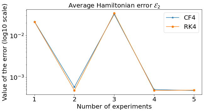
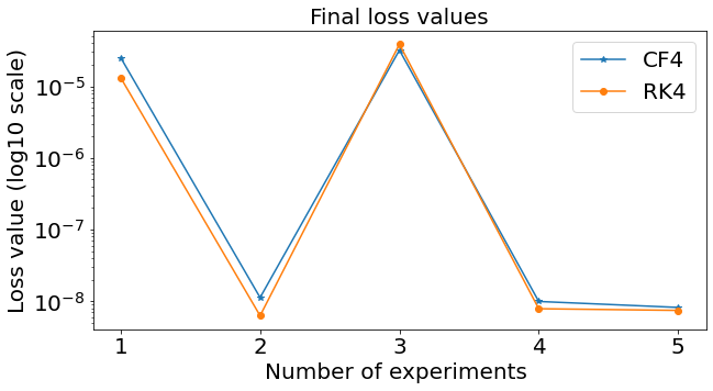
Measuring the approximation quality

\mathcal{E}_1 = \sum_{i=1}^{\bar{N}}\sum_{j=1}^{\bar{M}}\left\|z_i^j - \hat{z}_i^j\right\|^2

z_i^{j+1} = \tilde{\Psi}^{\Delta t}_{H}(z_i^j),\quad \hat{z}_i^{j+1} = \tilde{\Psi}^{\Delta t}_{H_{\theta}}(\hat{z}_i^j)

\mathcal{E}_{2}=\frac{1}{\bar{N}} \sum_{i=1}^{\bar{N}}\left|H\left(\bar{x}_{i}\right)-H_{\theta}\left(\bar{x}_{i}\right)-\frac{1}{\bar{N}} \sum_{l=1}^{\bar{N}}\left(H\left(\bar{x}_{i}\right)-H_{\theta}\left(\bar{x}_{i}\right)\right)\right|

\hat{z}_i^0 = z_i^0 = \bar{x}_i

Test initial conditions

Numerical experiment

H(q, p)=\frac{1}{2}\left[\begin{array}{ll} p_{1} & p_{2} \end{array}\right]^{T}\left[\begin{array}{cc} 5 & -1 \\ -1 & 5 \end{array}\right]\left[\begin{array}{l} p_{1} \\ p_{2} \end{array}\right]+\frac{q_{1}^{4}+q_{2}^{4}}{4}+\frac{q_{1}^{2}+q_{2}^{2}}{2}

⚠️ The integrator used in the test, can be different from the training one.

Physics informed regularization

If there is a known conserved quantity \(I(x(t))=I(x(0))\) we can add it to the loss, to get a physics informed regularization:

\mathcal{L}_{\theta}^R = \mathcal{L}_{\theta} + \gamma \sum_{i=1}^N\sum_{j=1}^M |I(\hat{y}_i^j)-I(x_i)|

H\left(x\right)=\frac{q_{1}^{2}+p_{1}^{2}}{2}+\frac{p_{2}^{2}}{2}+\frac{1}{2} q_{2}^{2}+\frac{1}{4} q_{2}^{4}\\ =h_{1}\left(q_{1}, p_{1}\right)+h_{2}\left(q_{2}, p_{2}\right)

\delta_i^j = \varepsilon n_i^j,\,n_i^j\sim \mathcal{N}(0,1)

I = h_1

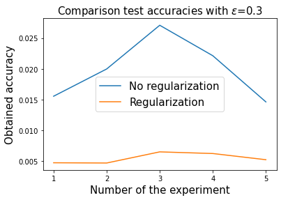
On clean trajectories

Constrained Hamiltonian systems

\begin{cases} \dot{x}(t) = \mathbb{J}\nabla H(q,p),\quad x=(q,p)\\ g(q) = 0,\quad g:\mathbb{R}^n\rightarrow\mathbb{R}^m \end{cases}

g(q)=0\implies G(q)\dot{q} = G(q)\partial_p H(q,p) = 0

This implies that the dynamics can be defined as a vector field on

\mathcal{M} = T^*\mathcal{Q}=T^*\{q\in\mathbb{R}^n:\,g(q)=0\} = \\ \{(q,p)\in\mathbb{R}^{2n}:\,g(q)=0,\,G(q)\partial_pH(q,p)=0\}

Modelling the vector field on \(\mathcal{M}\)

\mathcal{Q}=\{q\in\mathbb{R}^n:\;g(q)=0\}\subset\mathbb{R}^n,\\ dim\mathcal{Q}=n-m

P(q) : \mathbb{R}^n\rightarrow T_q\mathcal{Q},\,v\mapsto P(q)v

T_q\mathcal{Q} = \{v\in\mathbb{R}^n:\,G(q)v=0\}

\begin{cases} \dot{q}=P(q) \partial_{p} H(q, p) \\ \dot{p}=-P(q)^{T} \partial_{q} H(q, p)+W(q, p) \partial_{p} H(q, p) \end{cases}

On \(\mathcal{M}\) the dynamics can be written as

Example with \(\mathcal{Q}=S^2\)

\mathcal{Q}=\{q\in\mathbb{R}^3:\;\|q\|^2-1=0\}\subset\mathbb{R}^3,\\ dim\mathcal{Q}=2

P(q) : \mathbb{R}^3\rightarrow T_q\mathcal{Q},\,v\mapsto (I_3-qq^T)v

T_q\mathcal{Q} = \{v\in\mathbb{R}^3:\,q^Tv=0\}

\begin{cases} \dot{q} &=\left(I-q q^{T}\right) \partial_{p} H(q, p) \\ \dot{p} &=-\left(I-q q^{T}\right) \partial_{q} H(q, p)+\partial_{p} H(q, p) \times(p \times q) \end{cases}

On \(\mathcal{M}\) the dynamics can be written as

Learning constrained Hamiltonian systems

\hat{f}_{\theta}(q,p) = \begin{bmatrix} P(q) \partial_{p} H_{\theta}(q, p) \\ -P(q)^{T} \partial_{q} H_{\theta}(q, p)+W(q, p) \partial_{p} H_{\theta}(q, p) \end{bmatrix}

Proceed as in the general case, but the vector field \(\tilde{f}_{\theta}\) has a particular structure, as for the unconstrained case.

⚠️ \(\hat{f}_{\theta}\) makes sense also for \((q,p)\in\mathbb{R}^{2n}\setminus \mathcal{M}\), even if no more as a vector field on \(\mathcal{M}\)

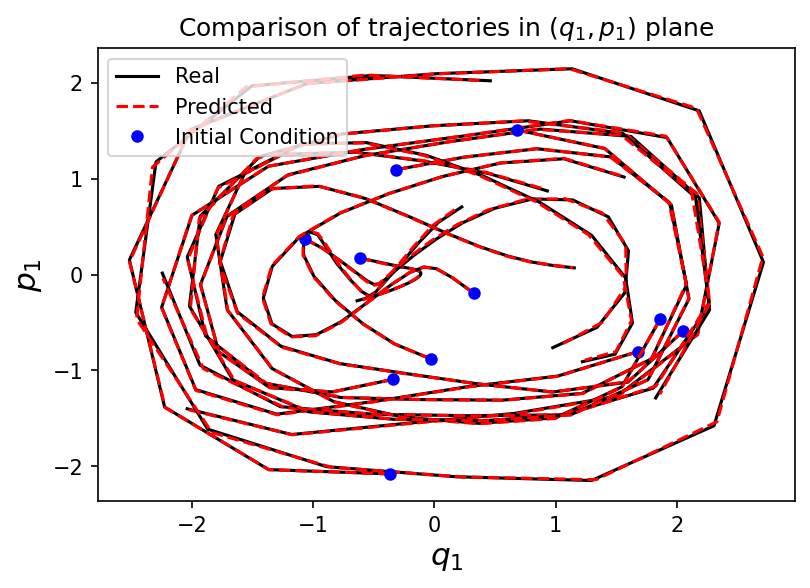
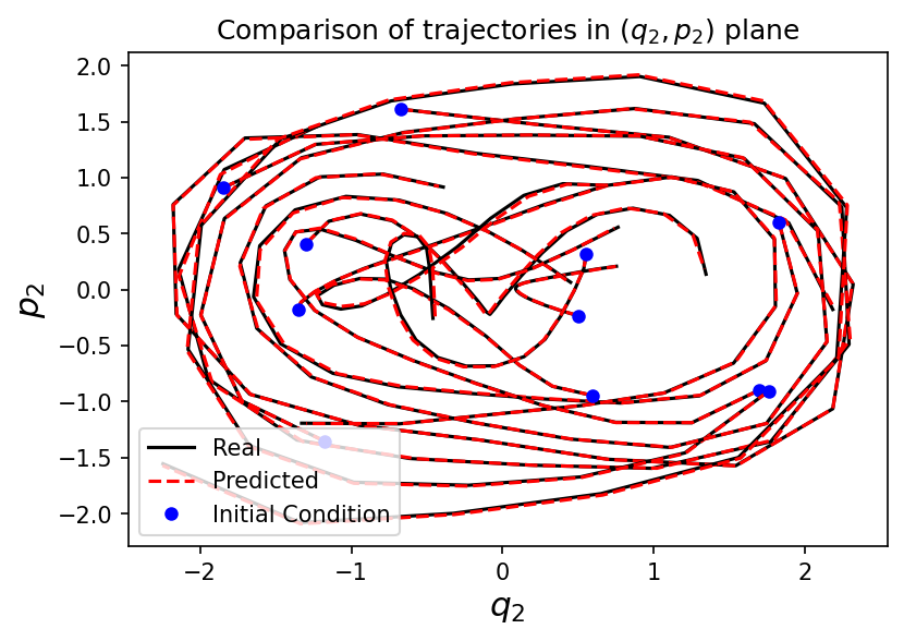
H_{\theta}(q, p)=\frac{1}{2} p^{T} M_{\theta_{1}}^{-1}(q) p+\operatorname{Net}_{\theta_{2}}(q), \\ \theta=\left(\theta_{1}, \theta_{2}\right)

Example with the double spherical pendulum

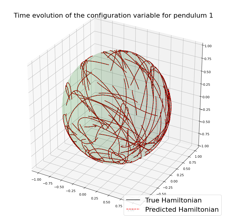
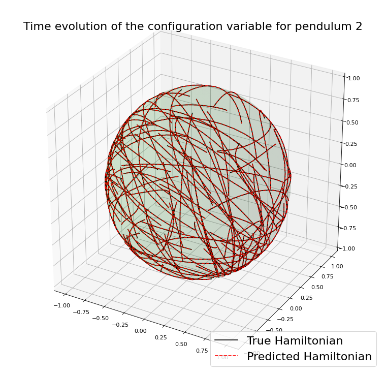
Using an integrator \(\Psi^{\Delta t}_{\theta}\) that preserves \(\mathcal{M}\)

PROS

CONS

On \(\mathcal{M}\) the function \(H_{\theta}\) is unique

The approximation error is not influenced by the drift from the manifold.

These methods are more involved, and often implicit.

The loss function can become harder to be optimized.

The simulated trajectories in the training are physically meaningful.

Not in general clear the impact this has on the final result.

Case with \(\mathcal{M}\) homogeneous

A manifold \(\mathcal{M}\) is homogeneous if there is a Lie group \(\mathcal{G}\) that defines a transitive group action \(\varphi:\mathcal{G}\times\mathcal{M}\rightarrow\mathcal{M}\).

Case with \(\mathcal{M}\) homogeneous

A manifold \(\mathcal{M}\) is homogeneous if there is a Lie group \(\mathcal{G}\) that defines a transitive group action \(\varphi:\mathcal{G}\times\mathcal{M}\rightarrow\mathcal{M}\).

A vector field \(f\) on \(\mathcal{M}\) can be represented as \(f(x) = \varphi_*(\xi(x))(x)\), for a function

\(\xi:\mathcal{M}\rightarrow\mathfrak{g}\simeq T_e\mathcal{G}\).

Lie Group Methods are a class of methods exploiting this structure and preserving \(\mathcal{M}\). The simplest is Lie Euler:

\(y_i^{j+1} = \varphi(\exp(\Delta t \,\xi(y_i^j)),y_i^j)\)

Basic idea of a class of Lie group methods

\(\mathcal{M}\)

\(y_i^j\)

\(y_i^{j+1}=\varphi_g(y_i^j)\)

\(\mathfrak{g}\)

\(\xi\)

\(\exp\)

\(\mathcal{G}\)

\(\varphi_g\)

\(\Psi^{\Delta t}\)

\(0\)

\(\Delta t \xi(y_i^j)\)

\(g=\exp(\Delta t\,\xi(y_i^j))\)

\(f\in\mathfrak{X}(M)\)

\(f^L\in\mathfrak{X}(\mathfrak{g})\)

A case where preserving \(\mathcal{M}\) helps

Suppose to have just few unknown elements in the expression of the Hamiltonian

As a consequence, one expects a very accurate approximation.

Example with the spherical pendulum:

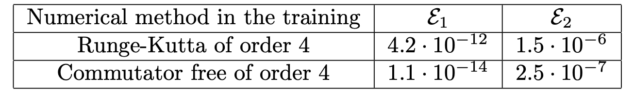
H_{\theta}(q, p)=\frac{1}{2 m} p^{T} p+u^{T} q, \quad m>0, u \in \mathbb{R}^{3}

Similar results preserving \(\mathcal{M}\)

N=500, M=3, T=0.1, n=3

System studied: Spherical pendulum

Thank you for the attention

Slides available at

https://slides.com/davidemurari/constrained-hamiltonian