Learning Hamiltonians of constrained systems

Learning Hamiltonians of constrained mechanical systems

Davide Murari

One day – Young Researchers Seminars, Maths Applications & Models

\(\texttt{davide.murari@ntnu.no}\)

Joint work with Elena Celledoni, Andrea Leone and Brynjulf Owren

Definition of the problem

\dot{x}(t) = f(x(t))\in\mathbb{R}^m

GOAL : approximate the unknown \(f\) on \(\Omega\)

DATA:

\{(x_i,y_i^1,...,y_i^M)\}_{i=1,...,N},\\ x_i\in\Omega\subset\mathbb{R}^m

y_i^j = \Phi_f^{j\Delta t}(x_i) + \delta_i^j

\Delta t>0

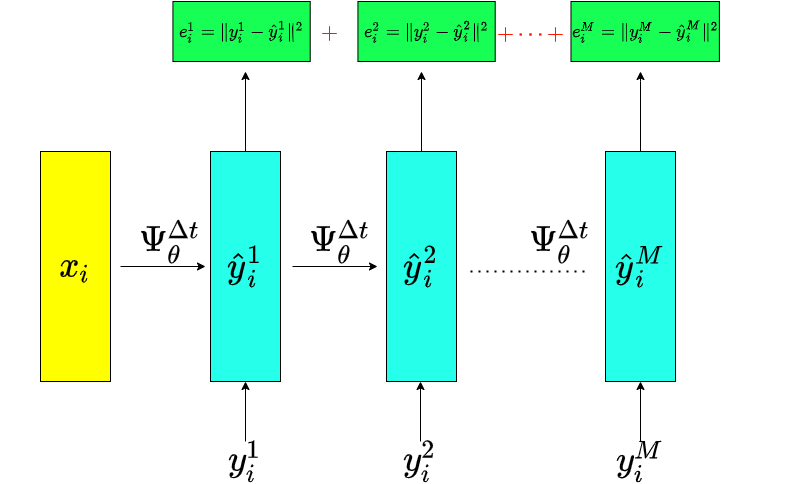
Approximation of a dynamical system

Introduce a parametric model

\dot{x}(t) = \hat{f}_{\theta}(x(t))

\text{solve}\quad \min_{\theta} \sum_{i=1}^N \sum_{j=1}^M \left\|y_i^j - \hat{y}_i^{j}\right\|^2 = \min_{\theta}\mathcal{L}_{\theta}

1️⃣

3️⃣

Choose any numerical integrator applied to \(\hat{f}_{\theta}\)

\hat{y}_i^0 = x_i,\,\,\hat{y}_i^{j+1} = \Psi_{\theta}^{\Delta t}(\hat{y}_i^{j})

2️⃣

\mathcal{L}_i

Unconstrained Hamiltonian systems

f(q,p) = \mathbb{J}\nabla H(q,p)=\begin{bmatrix} \partial_p H(q,p) \\ -\partial_q H(q,p)\end{bmatrix},

H:\mathbb{R}^{2n}\rightarrow\mathbb{R},\quad \mathbb{J} = \begin{bmatrix} 0_n & I_n \\ -I_n & 0_n \end{bmatrix}\in\mathbb{R}^{2n\times 2n}

Unconstrained Hamiltonian systems

f(q,p) = \mathbb{J}\nabla H(q,p)=\begin{bmatrix} \partial_p H(q,p) \\ -\partial_q H(q,p)\end{bmatrix},

H:\mathbb{R}^{2n}\rightarrow\mathbb{R},\quad \mathbb{J} = \begin{bmatrix} 0_n & I_n \\ -I_n & 0_n \end{bmatrix}\in\mathbb{R}^{2n\times 2n}

Choice of the model:

\hat{f}_{\theta}(q,p) = \mathbb{J}\nabla H_{\theta}(q,p)

H_{\theta}(q,p) = \frac{1}{2}p^TA^TAp + Net_{\bar{\theta}}(q),\quad \theta = (A,\bar{\theta})

\(Net_{\bar{\theta}}(q)\)

Net_{\bar{\theta}}(q) = \mathcal{N}_{\bar{\theta}_k} \circ ... \circ \mathcal{N}_{\bar{\theta}_1}(q)

\mathcal{N}_{\bar{\theta}_i}(q) = \Sigma(A_iq + b_i)

\Sigma(q) = [\sigma(q_1),...,\sigma(q_n)],\\ \sigma:\mathbb{R}\rightarrow\mathbb{R}

Measuring the approximation quality

\mathcal{E}_1 = \sum_{i=1}^{\bar{N}}\sum_{j=1}^{\bar{M}}\left\|z_i^j - \hat{z}_i^j\right\|^2

z_i^{j+1} = \tilde{\Psi}^{\Delta t}_{H}(z_i^j),\quad \hat{z}_i^{j+1} = \tilde{\Psi}^{\Delta t}_{H_{\theta}}(\hat{z}_i^j)

\mathcal{E}_{2}=\frac{1}{\bar{N}} \sum_{i=1}^{\bar{N}}\left|H\left(\bar{x}_{i}\right)-H_{\theta}\left(\bar{x}_{i}\right)-\frac{1}{\bar{N}} \sum_{l=1}^{\bar{N}}\left(H\left(\bar{x}_{l}\right)-H_{\theta}\left(\bar{x}_{l}\right)\right)\right|

\hat{z}_i^0 = z_i^0 = \bar{x}_i

Test initial conditions

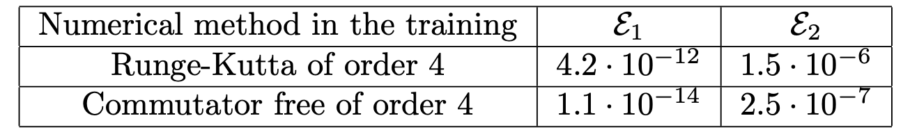
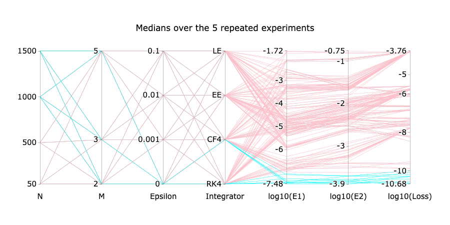
Numerical experiment

H(q, p)=\frac{1}{2}\left[\begin{array}{ll} p_{1} & p_{2} \end{array}\right]^{T}\left[\begin{array}{cc} 5 & -1 \\ -1 & 5 \end{array}\right]\left[\begin{array}{l} p_{1} \\ p_{2} \end{array}\right]+\frac{q_{1}^{4}+q_{2}^{4}}{4}+\frac{q_{1}^{2}+q_{2}^{2}}{2}

⚠️ The integrator used in the test, can be different from the training one.

Constrained Hamiltonian systems

\begin{cases} \dot{x}(t) = \mathbb{J}\nabla H(q,p),\quad x=(q,p)\\ g(q) = 0,\quad g:\mathbb{R}^n\rightarrow\mathbb{R}^m \end{cases}

\mathcal{M} = T^*\mathcal{Q}=T^*\{q\in\mathbb{R}^n:\,g(q)=0\} = \\ \{(q,p)\in\mathbb{R}^{2n}:\,g(q)=0,\,G(q)\partial_pH(q,p)=0\}

\mathcal{Q}=\{q\in\mathbb{R}^n:\;g(q)=0\}\subset\mathbb{R}^n

Modelling the vector field on \(\mathcal{M}\)

P(q) : \mathbb{R}^n\rightarrow T_q\mathcal{Q},\,v\mapsto P(q)v

T_q\mathcal{Q} = \{v\in\mathbb{R}^n:\,G(q)v=0\}

\begin{cases} \dot{q}=P(q) \partial_{p} H(q, p) \\ \dot{p}=-P(q)^{T} \partial_{q} H(q, p)+W(q, p) \partial_{p} H(q, p) \end{cases}

On \(\mathcal{M}\) the dynamics can be written as

⚠️ On \(\mathbb{R}^{2n}\setminus\mathcal{M}\) the vector field extends non-uniquely.

Learning constrained Hamiltonian systems

\hat{f}_{\theta}(q,p) = \begin{bmatrix} P(q) \partial_{p} H_{\theta}(q, p) \\ -P(q)^{T} \partial_{q} H_{\theta}(q, p)+W(q, p) \partial_{p} H_{\theta}(q, p) \end{bmatrix}

H_{\theta}(q, p)=\frac{1}{2} p^{T} M_{\theta_{1}}^{-1}(q) p+\operatorname{Net}_{\theta_{2}}(q), \\ \theta=\left(\theta_{1}, \theta_{2}\right)

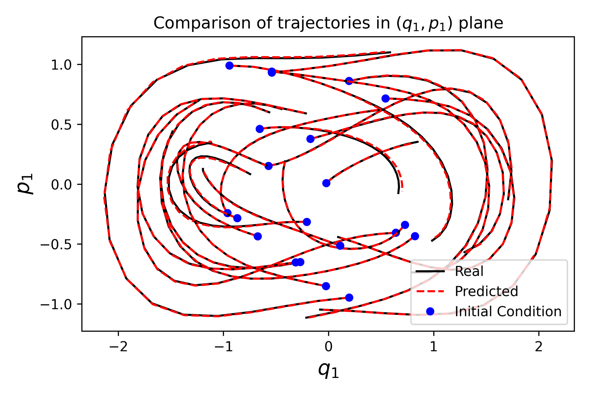
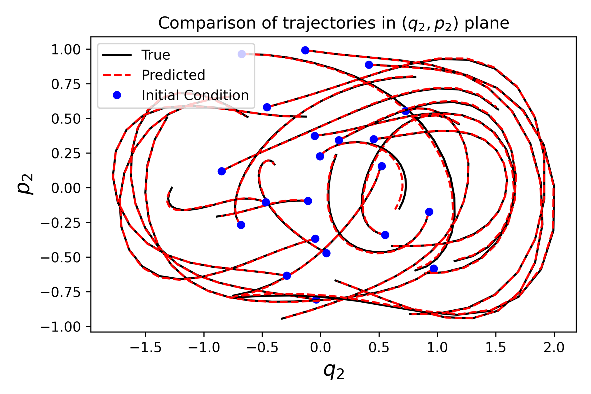
Example with the double spherical pendulum

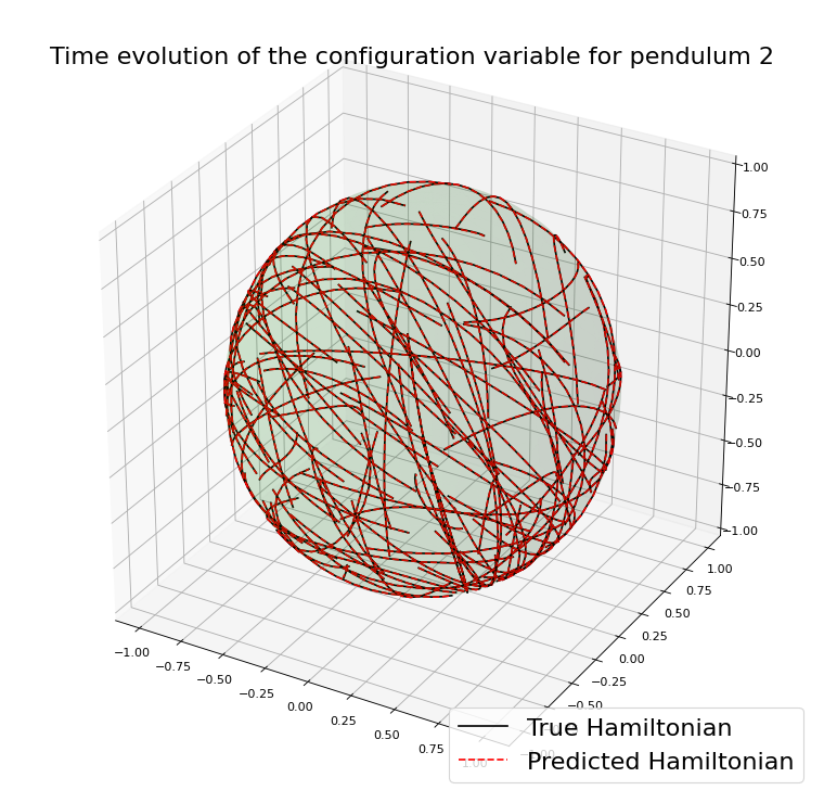
A case where preserving \(\mathcal{M}\) helps

Suppose to have just few unknown elements in the expression of the Hamiltonian

As a consequence, one expects a very accurate approximation.

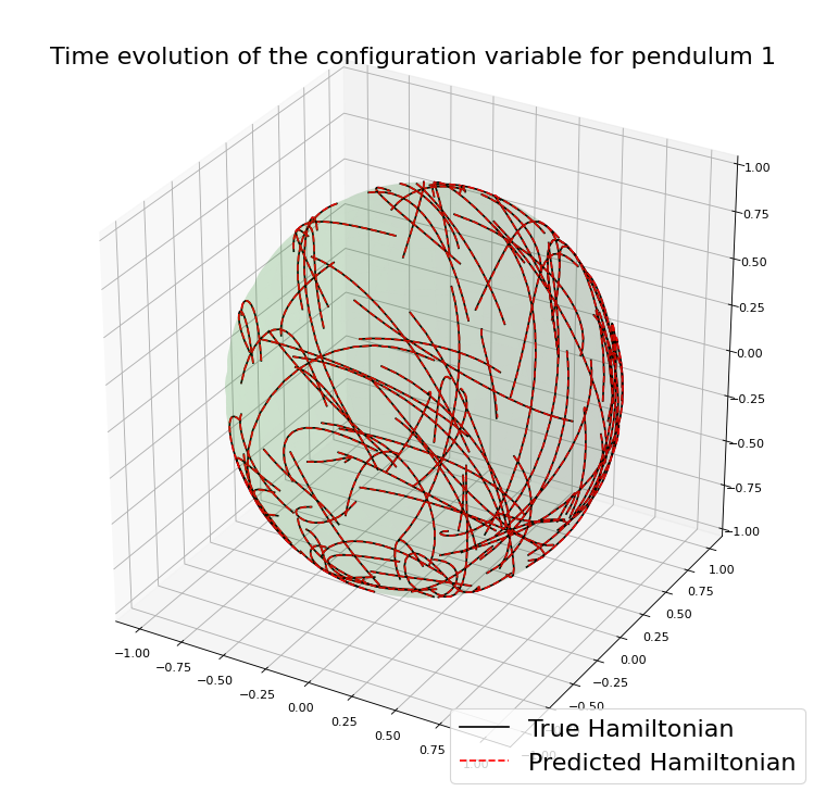
Example with the spherical pendulum:

H_{\theta}(q, p)=\frac{1}{2 m} p^{T} p+u^{T} q, \quad m>0, u \in \mathbb{R}^{3}

Similar results preserving \(\mathcal{M}\)

For interactive plots complementary

to this:

Thank you for the attention

Preprint:

Celledoni, E., Leone, A., Murari, D., & Owren, B. (2022). Learning Hamiltonians of constrained mechanical systems. arXiv preprint arXiv:2201.13254