Neural networks modelled by dynamical systems

Davide Murari

DNA Seminar - 20/06/2022

\(\texttt{davide.murari@ntnu.no}\)

Joint work with Elena Celledoni, Brynjulf Owren,

Carola-Bibiane Schönlieb and Ferdia Sherry

Outline

What is supervised learning

Consider two sets \(\mathcal{C}\) and \(\mathcal{D}\) and suppose to be interested in a specific (unknown) mapping \(F:\mathcal{C}\rightarrow \mathcal{D}\).

The data we have available can be of two types:

Direct measurements of \(F\): \(\mathcal{T} = \{(x_i,y_i=F(x_i)\}_{i=1,...,N}\subset\mathcal{C}\times\mathcal{D}\)
Indirect measurements that characterize \(F\): \(\mathcal{I} = \{(x_i,z_i=G(F(x_i))\}_{i=1,...,N}\subset\mathcal{C}\times G(\mathcal{D})\)

GOAL: Approximate \(F\) on all \(\mathcal{C}\).

What are neural networks

Source image: https://www.tibco.com/reference-center/what-is-a-neural-network

What are neural networks

They are compositions of parametric functions

\( \mathcal{NN}(x) = f_{\theta_k}\circ ... \circ f_{\theta_1}(x)\)

Examples

\(f_{\theta}(x) = x + B\Sigma(Ax+b),\quad \theta = (A,B,b)\)

ResNets

Feed Forward

Networks

\(f_{\theta}(x) = B\Sigma(Ax+b),\quad \theta = (A,B,b)\)

\(\Sigma(z) = [\sigma(z_1),...,\sigma(z_n)],\quad \sigma:\mathbb{R}\rightarrow\mathbb{R}\)

Neural networks modelled by dynamical systems

\mathcal{NN}(x) = \Psi_{f_k}^{h_k}\circ ...\circ \Psi_{f_1}^{h_1}(x)

EXPLICIT

EULER

\( \Psi_{f_i}^{h_i}(x) = x + h_i f_i(x)\)

\( \dot{x}(t) = f(t,x(t),\theta(t)) \)

Time discretization : \(0 = t_1 < ... < t_k <t_{k+1}= T \), \(h_i = t_{i+1}-t_{i}\)

Where \(f_i(x) = f(t_i,x,\theta(t_i))\)

EXAMPLE

\(\dot{x}(t) = \Sigma(A(t)x(t) + b(t))\)

Imposing some structure

\dot{x}(t) = \left[A(t,x(t))-A^T(t,x(t))\right]\boldsymbol{1}

\dot{x}(t) = \mathbb{J}A^T(t)\Sigma(A(t)x(t)+b(t))

\ddot{x}(t) = \Sigma(A(t)x(t)+b(t))

MASS PRESERVING NETWORKS

HAMILTONIAN NETWORKS

VOLUME PRESERVING, INVERTIBLE

Approximation result

f_i(x) = \nabla U_i(x) + X_S^i(x)

U_i(x) = \int_0^1 x^Tf_i(tx)dt

x^TX_S^i(x)=0\quad \forall x\in\mathbb{R}^n

Then \(F\) can be approximated arbitrarily well by composing flow maps of gradient and sphere preserving vector fields.

F:\Omega\subset\mathbb{R}^n\rightarrow\mathbb{R}^n\quad \text{continuous}

\forall \varepsilon>0\,\,\exist f_1,…,f_k\in\mathcal{C}^1(\mathbb{R}^n,\mathbb{R}^n)\,\,\text{s.t.}

\|F-\Phi_{f_k}^{h_k}\circ … \circ \Phi_{f_1}^{h_1}\|<\varepsilon

Approximation result

\Phi_{f_i}^h = \Phi_{f_i}^{\alpha_M h} \circ ... \circ \Phi_{f_i}^{\alpha_1 h}

\sum_{i=1}^M \alpha_i = 1

f = \nabla U + X_S \\ \implies \Phi_f^h(x) = \Phi_{\nabla U}^{h/2} \circ \Phi_{X_S}^h \circ \Phi_{\nabla U}^{h/2}(x) + \mathcal{O}(h^3)

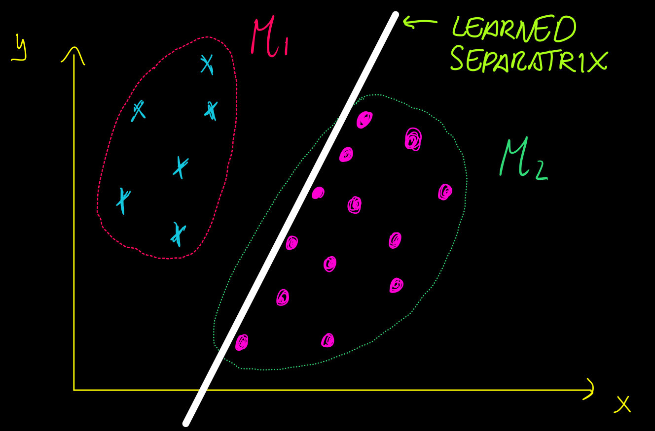
The classification problem

Given a "sufficiently large" set of \(N\) points in \(\mathcal{M}\subset\mathbb{R}^k\) that belong to \(C\) classes, we want to learn a function \(F\) assigning all the points of \(\mathcal{M}\) to the correct class.

F : \mathbb{R}^k \rightarrow \mathbb{R}^C

\ell_F(x):=\arg\max\{F(x)_j:j=1,...,C\} = i=:\ell(x) \\ \forall x\in \mathcal{M}_i

\mathcal{M} = \bigcup\limits_{i=1}^C \mathcal{M}_i \subset \mathbb{R}^k

Adversarial examples

\text{Find }\eta\in\mathbb{R}^k\\ \text{s.t.}\,\,\|\eta\|\leq \varepsilon,\,\,\ell_F(x)\neq \ell_F(x+\eta)

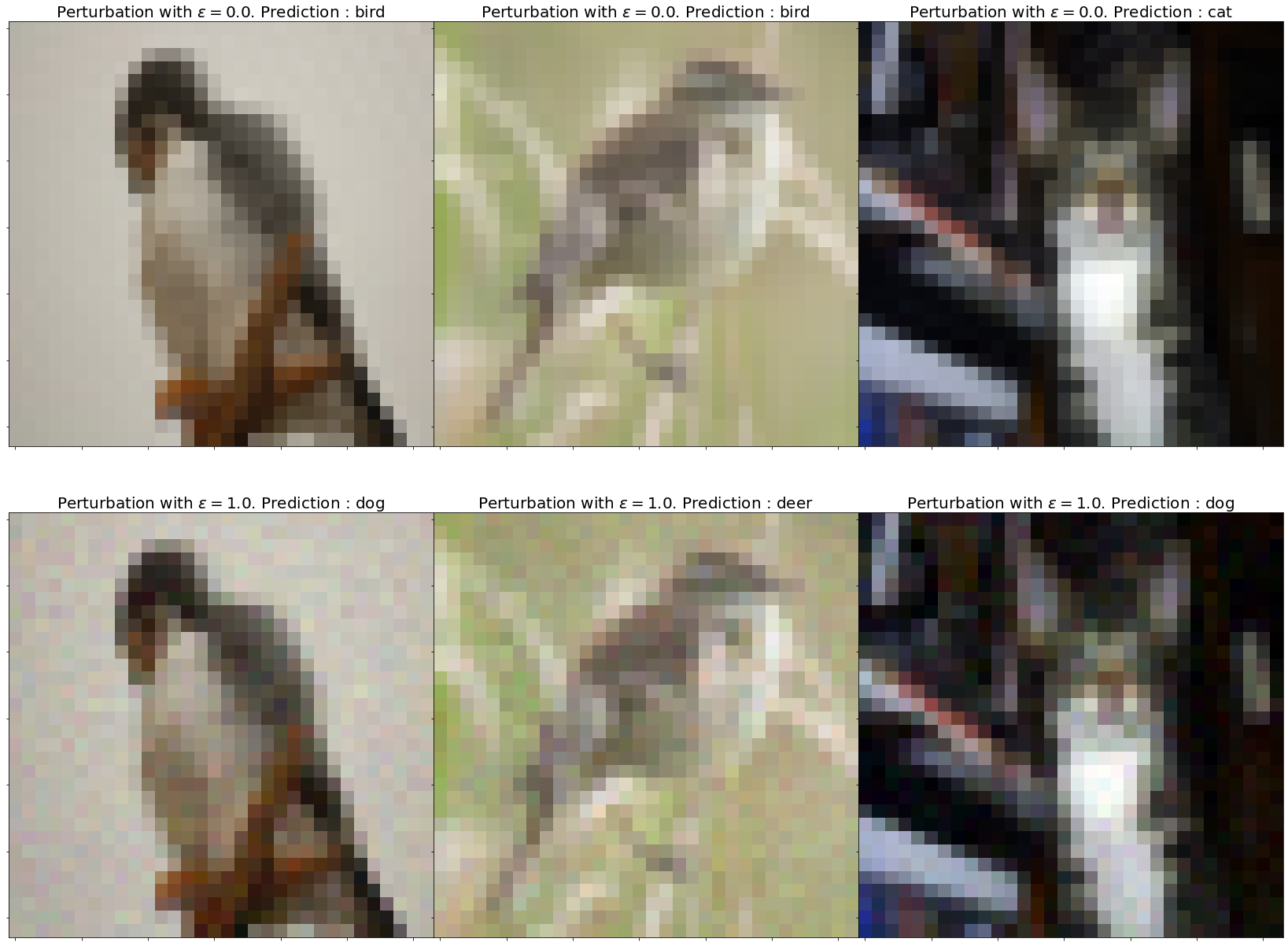
What is a robust classifier?

An \(\varepsilon\)-robust classifier is a function that not only correctly classifies the points in \(\mathcal{M}\) but also those in

Suppose that

d(\mathcal{M_i},\mathcal{M}_j)>2\varepsilon\quad \forall i\neq j

\mathcal{M}_{\varepsilon} := \{x\in\mathbb{R}^k\,:\,d(x,\mathcal{M})\leq \varepsilon\}

\ell_F(x) = i := \ell(x) \quad \forall x\in \mathcal{M}_i

\ell_F(x+\eta) = i\;\; \forall x\in \mathcal{M}_i,\|\eta\|\leq \varepsilon

In other words, we should learn a

F : \mathbb{R}^k \rightarrow \mathbb{R}^C

such that

Sensitivity measures for \(F\)

\|F(x+\eta)-F(x)\|\leq \text{Lip}(F)\|\eta\|

Idea:

"GOOD"

[0.99, 0.05, 0.05]

"BAD"

[0.34, 0.33, 0.33]

M_F(x) := \max\{0,F(x)_{i} - \max_{j\neq i} F(x)_j\}\\ \ell(x)=i

How to have guaranteed robustness

M_F(x)\geq \sqrt{2}\text{Lip}(F)\varepsilon \\ \implies \ell_F(x) = \ell_F(x+\eta)\,\forall \|\eta\|\leq \varepsilon

\mathcal{L} = \frac{1}{N}\sum_{i=1}^N \sum_{j\neq \ell(x)} \max\{0,m-(F(x)_{\ell(x)}-F(x)_j)\}

1️⃣

2️⃣

We constrain the Lipschitz constant of \(F\)

Lipschitz networks based on dynamical systems

\Gamma(x) = [\gamma(x_1),...,\gamma(x_k)]\\ V_{\theta} = \boldsymbol{1}^T\Gamma(Ax+b),\,\,\theta =[A,b]\\ X_{\theta}^{\pm}(z) := \pm \nabla V_{\theta}(z)

\mu_{\theta} \|z-y\|^2\leq\langle \nabla V_{\theta}(z)- \nabla V_{\theta}(y),z-y\rangle\leq L_{\theta}\|x-y\|^2\\ \implies \|\Phi^{t}_{\nabla V_{\theta}}(x)-\Phi^{t}_{\nabla V_{\theta}}(y)\|\leq e^{L_{\theta} t} \|x-y\|\\ \implies \|\Phi^{t}_{-\nabla V_{\theta}}(x)-\Phi^{t}_{-\nabla V_{\theta}}(y)\|\leq e^{-\mu_{\theta} t} \|x-y\|

Lipschitz networks based on dynamical systems

F(x) \approx F_{\theta}(x)=\Phi_{-\nabla V_{\theta_{2k}}}^{h_{2k}} \circ \Phi_{\nabla V_{\theta_{2k-1}}}^{h_{2k-1}} \circ ... \circ \Phi_{-\nabla V_{\theta_2}}^{h_2} \circ \Phi_{\nabla V_{\theta_{1}}}^{h_1}(x)

\|F_{\theta}(x)-F_{\theta}(y)\|\leq \exp\left(\sum_{i=1}^k \gamma_i\right)\|x-y\|

\exp\left(\sum_{i=1}^k \gamma_i\right)

\gamma_i = h_{2i-1}L_{\theta_{2i-1}} - h_{2i}\mu_{\theta_{2i}}

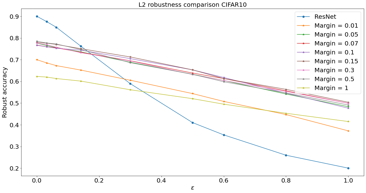
Adversarial robustness

Thank you for the attention