Structured neural networks and some applications to dynamical systems

Davide Murari

davide.murari@ntnu.no

In collaboration with : Elena Celledoni, Andrea Leone, Brynjulf Owren, Carola-Bibiane Schönlieb, and Ferdia Sherry

FoCM, 12 June 2023

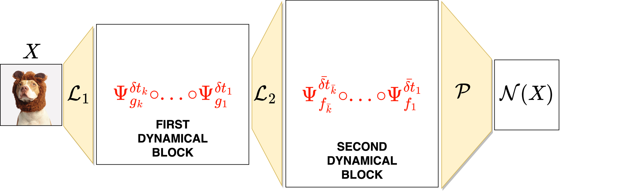
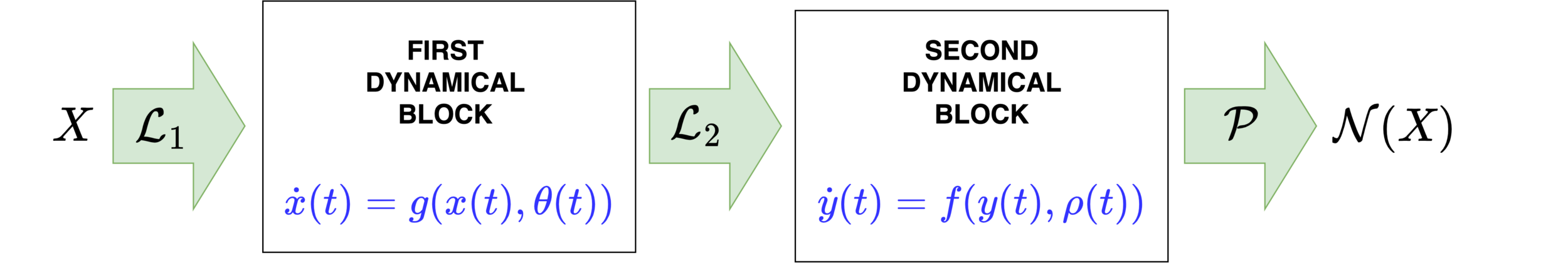
\( \mathcal{N}(x) = f_{\theta_M}\circ ... \circ f_{\theta_1}(x)\)

Neural networks motivated by dynamical systems

\( \mathcal{N}(x) = f_{\theta_M}\circ ... \circ f_{\theta_1}(x)\)

Neural networks motivated by dynamical systems

\( \dot{x}(t) = f(x(t),\theta(t)) \)

\( \delta t_i = t_{i}-t_{i-1}\)

t_0

t_1

t_2

t_i

t_{i+1}

t_M

\cdots

\( \mathcal{N}(x) = f_{\theta_M}\circ ... \circ f_{\theta_1}(x)\)

Neural networks motivated by dynamical systems

t_0

t_1

t_2

t_i

t_{i+1}

t_M

\cdots

\mathcal{N}(x) = \Psi_{f_M}^{\delta t_M}\circ ...\circ \Psi_{f_1}^{\delta t_1}(x)

\( \dot{x}(t) = f(x(t),\theta(t)) \)

Where \(f_i(x) = f(x,\theta(t_i))\)

\( \delta t_i = t_{i}-t_{i-1}\)

Neural networks motivated by dynamical systems

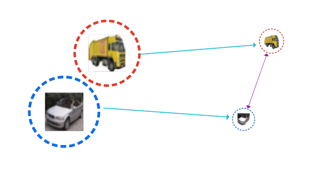
Accuracy is not everything

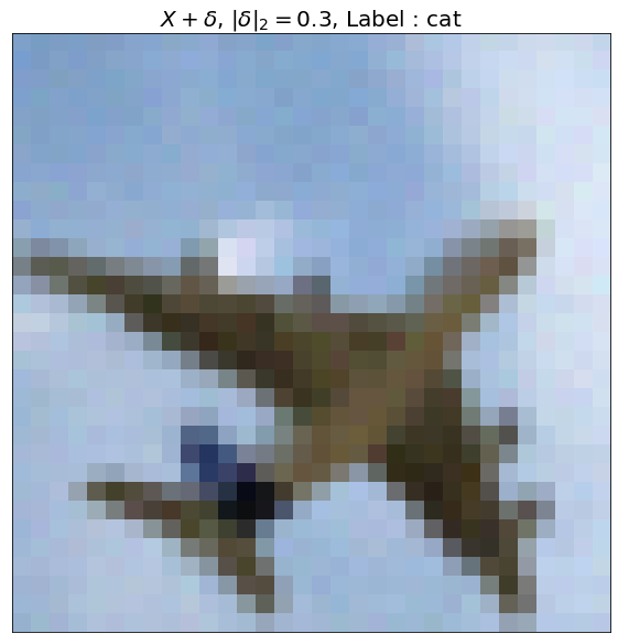
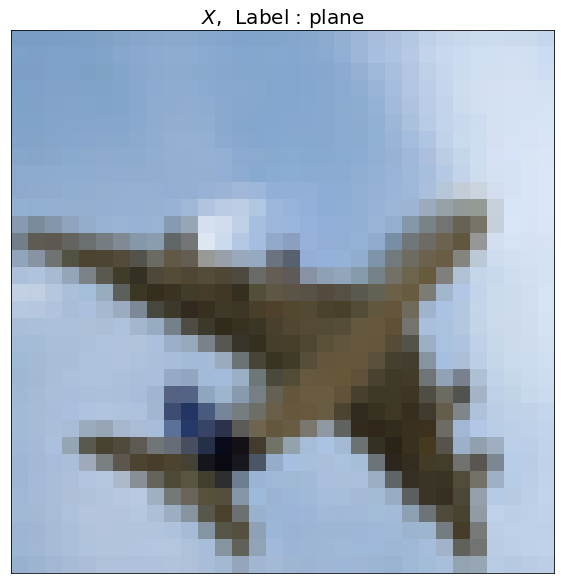
\(X\) , Label : Plane

\(X+\delta\), \(\|\delta\|_2=0.3\) , Label : Cat

Informed network design

GENERAL IDEA

EXAMPLE

Property \(\mathcal{P}\)

\(\mathcal{P}=\) Volume preservation

\mathcal{N}(x) = \Psi_{f_M}^{\delta t_M}\circ ...\circ \Psi_{f_1}^{\delta t_1}(x)

Family \(\mathcal{F}\) of vector fields that satisfy \(\mathcal{P}\)

\(f_{\theta}(x,v) = \begin{bmatrix} \Sigma(Av+a) \\ \Sigma(Bx+b) \end{bmatrix} \)

\(\mathcal{F}=\{f_{\theta}:\,\,\theta\in\Theta\}\)

Informed network design

\mathcal{N}(x) = \Psi_{f_M}^{\delta t_M}\circ ...\circ \Psi_{f_1}^{\delta t_1}(x)

GENERAL IDEA

EXAMPLE

Property \(\mathcal{P}\)

\(\mathcal{P}=\) Volume preservation

Integrator \(\Psi^{\delta t}\) that preserves \(\mathcal{P}\)

x_{n+1}=x_n+\delta t\Sigma(A_nv_n+a_n)\\ v_{n+1}=v_n+\delta t\Sigma(B_nx_{n+1}+b_n)\\ (x_{n+1},v_{n+1}) = \Psi^{\delta t}_{f_{\theta_n}}(x_n,v_n)

Informed network design

\mathcal{N}(x) = \Psi_{f_M}^{\delta t_M}\circ ...\circ \Psi_{f_1}^{\delta t_1}(x)

Family \(\mathcal{F}\) of vector fields that satisfy \(\mathcal{P}\)

\(f_{\theta}(x,v) = \begin{bmatrix} \Sigma(Av+a) \\ \Sigma(Bx+b) \end{bmatrix} \)

\(\mathcal{F}=\{f_{\theta}:\,\,\theta\in\Theta\}\)

GENERAL IDEA

EXAMPLE

Property \(\mathcal{P}\)

\(\mathcal{P}=\) Volume preservation

Non-expansive neural

networks

\(\mathcal{N}_{\theta}\)

Margin

\(B_{\delta}(X)\)

\(B_{\gamma}(Y)\)

\(B_{\gamma'}(\mathcal{N}_{\theta}(Y))\)

\(B_{\delta'}(\mathcal{N}_{\theta}(X))\)

\(X\)

\(Y\)

\mathbb{R}^{3\times 32\times 32}

\mathbb{R}^{10}

\delta'<\delta,\,\,\gamma'<\gamma

Building blocks of the network

f_{\theta_i}(x) := - \nabla V_{\theta_i}(x) = -A_i^T\Sigma(A_ix+b_i)

\Psi^{\delta t_C}_{f_{\theta_i}}(x) = x - {\delta t_C}A_i^T\Sigma(A_ix+b_i)

g_{\theta_i}(x) := W_i^T\Sigma(W_ix + v_i)

\|\Psi^{\delta t_C}_{f_{\theta_i}}(y) - \Psi^{\delta t_C}_{f_{\theta_i}}(x)\|\leq \sqrt{1-{\delta t_C}+{\delta t_C}^2}\|y-x\|

\Psi^{\delta t_E}_{g_{\theta_i}}(x) = x + {\delta t_E}W_i^T\Sigma(W_ix+v_i)

\|\Psi^{\delta t_E}_{g_{\theta_i}}(y) - \Psi^{\delta t_E}_{g_{\theta_i}}(x)\|\leq (1+{\delta t_E})\|y-x\|

\mathcal{N}_{\theta}(x)=\Psi_{f_{\theta_{2k}}}^{\delta t_{2k}} \circ \Psi_{g_{\theta_{2k-1}}}^{\delta t_{2k-1}} \circ ... \circ \Psi_{f_{\theta_2}}^{\delta t_2} \circ \Psi_{g_{\theta_{1}}}^{\delta t_1}(x)

We impose :

\|\mathcal{N}_{\theta}(x)-\mathcal{N}_{\theta}(y)\|\leq \|x-y\|

\sqrt{1-{\delta t_{2i}}+{\delta t_{2i}}^2}(1+\delta t_{2i-1})\leq 1,\,\,i=1,...,k

Non-expansivity constraint

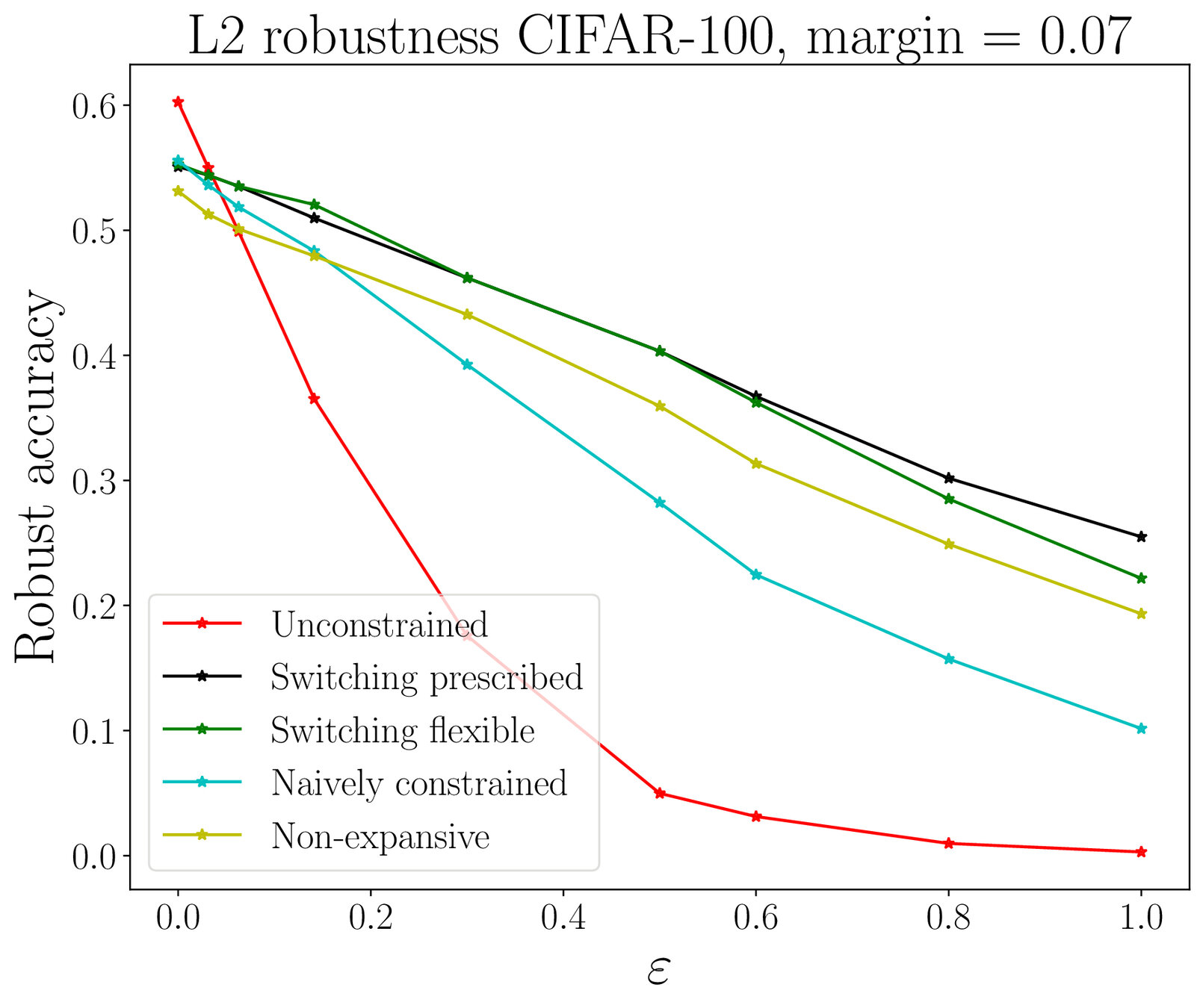
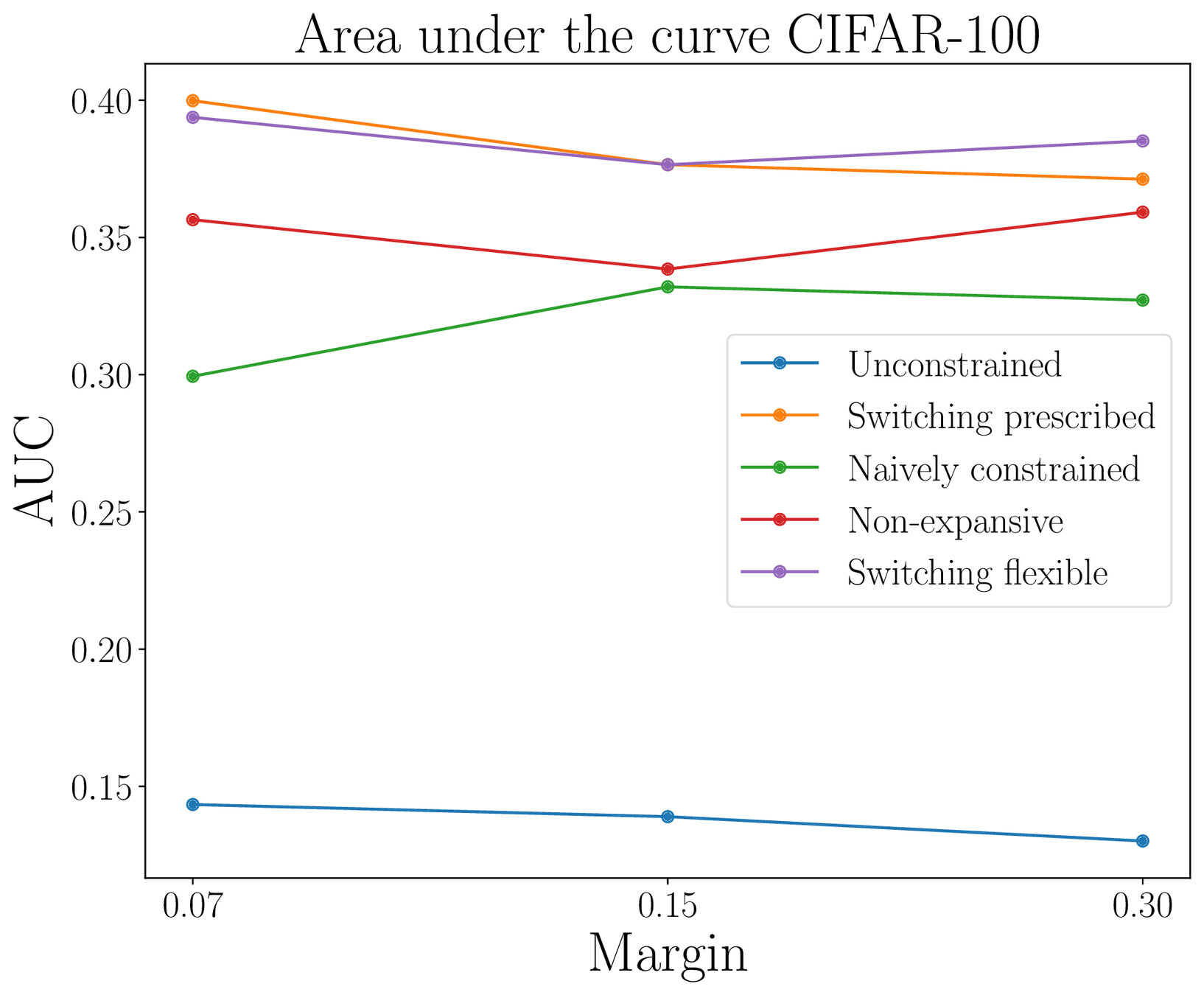
Adversarial robustness

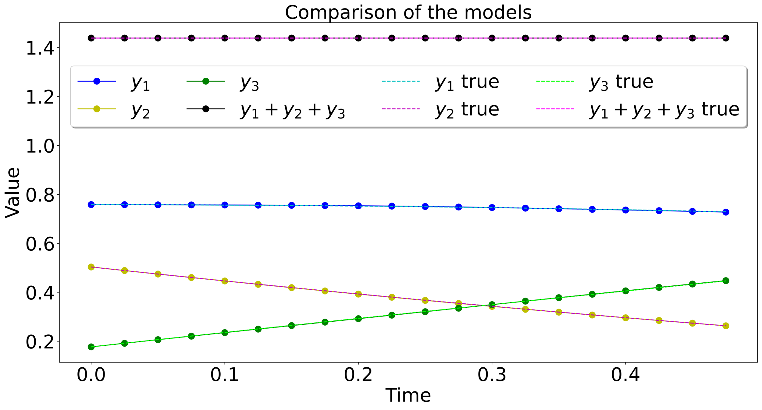
Approximating constrained mechanical systems

Data : \(\{(y_i^0,...,y_i^M)\}_{i=1,...,N}\)

\(y_i^{j} = \Phi^{j\delta t}_{Y}(y_i^0) + \varepsilon_i^j\in\mathbb{R}^n\)

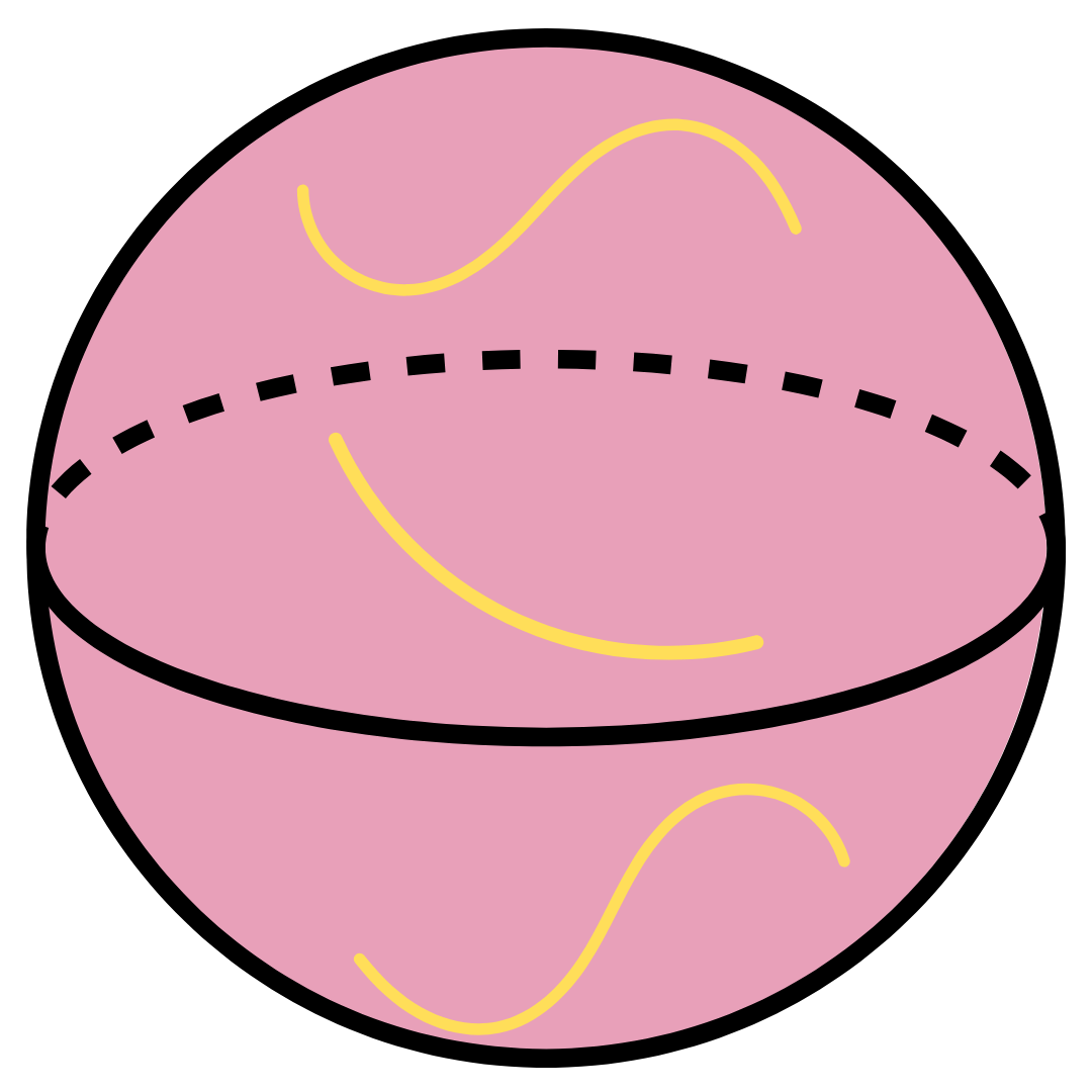
\(Y\in\mathfrak{X}(\mathcal{M})\) and

\(\delta t>0\) unknown

Goal : Approximate the map \(\Phi^{\delta t}_Y\)

\(\mathcal{M}\subset\mathbb{R}^n\)

\(y_1^0\)

\(y_1^1\)

\(y_1^2\)

\(y_1^3\)

\(y_2^0\)

\(y_2^1\)

\(y_2^2\)

\(y_2^3\)

\(y_3^0\)

\(y_3^1\)

\(y_3^2\)

\(y_3^3\)

A possible approach

\(\mathcal{N}_{\theta}:=\Psi^h_{Y_{\theta}}\circ ... \circ \Psi^h_{Y_{\theta}}\)

\(\theta = \arg\min_{\rho} \sum_{i=1}^N\sum_{j=1}^M\left\|y_i^j -\mathcal{N}_{\rho}^j(y_i^0)\right\|^2\)

\mathcal{M}

\mathbb{R}^n

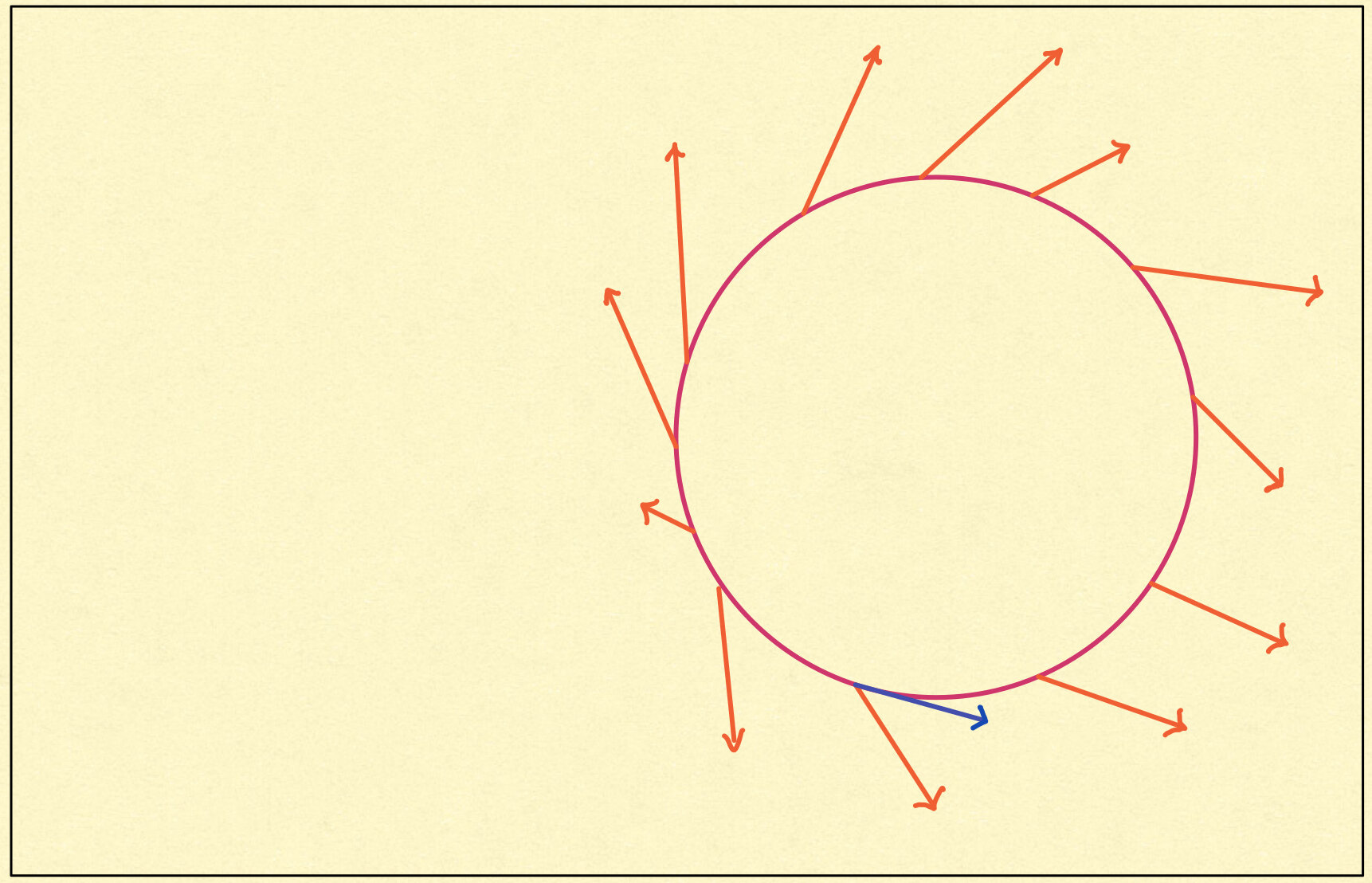
\(P(q) : \mathbb{R}^n\rightarrow T_q\mathcal{M},\, q\in\mathcal{M}\)
\(X_{\theta}\in\mathfrak{X}(\mathbb{R}^n)\)
\(Y_{\theta}(q) = P(q)X_{\theta}(q)\in T_q \mathcal{M}\)
\(\Psi_{Y_{\theta}}^h : \mathcal{M}\rightarrow\mathcal{M}\)

\(X_{\theta}(q)\)

\(q\)

\(Y_{\theta}(q)\)

Hamiltonian case

\Pi(q) : \mathbb{R}^n\rightarrow T_q\mathcal{Q},\,v\mapsto \Pi(q)v

T_q\mathcal{Q} = \{v\in\mathbb{R}^n:\,G(q)v=0\}

\begin{cases} \dot{q}=\Pi(q) \partial_{p} H(q, p) \\ \dot{p}=-\Pi(q)^{T} \partial_{q} H(q, p)+W(q, p) \partial_{p} H(q, p) \end{cases}

⚠️ On \(\mathbb{R}^{2n}\setminus\mathcal{M}\) the vector field extends non-uniquely.

\mathcal{Q} = \{q\in\mathbb{R}^n:\,G(q)=0\},\,\, \mathcal{M} = T^*\mathcal{Q}\subset\mathbb{R}^{2n}

Hamiltonian case

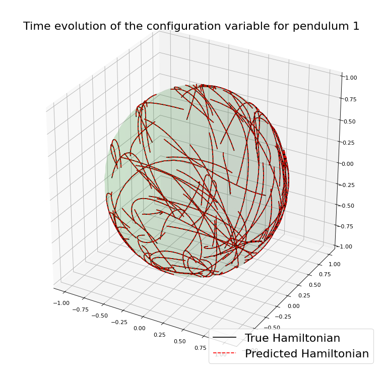
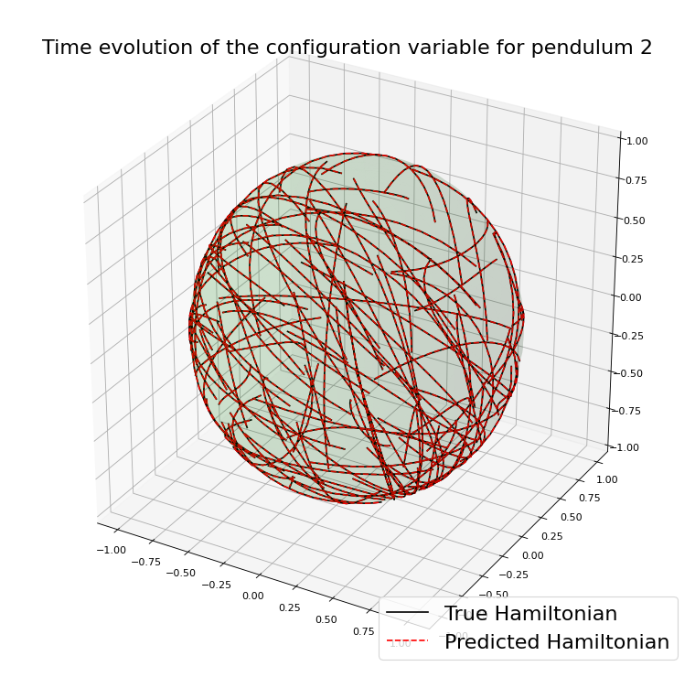
Y_{\theta}(q,p) = \begin{bmatrix} \Pi(q) \partial_{p} H_{\theta}(q, p) \\ -\Pi(q)^{T} \partial_{q} H_{\theta}(q, p)+W(q, p) \partial_{p} H_{\theta}(q, p) \end{bmatrix}

H_{\theta}(q, p)=\frac{1}{2} p^{T} M_{\theta_{1}}^{-1}(q) p+\mathcal{N}_{\theta_{2}}(q), \\ \mathcal{N}_{\theta_2}(q) = f_{\rho_m}\circ ... \circ f_{\rho_1}(q)\\ \theta=\left(\theta_{1}, \theta_{2}\right),\,\,\theta_2=(\rho_1,...,\rho_m)

Double spherical pendulum

\mathcal{Q} = \mathcal{S}^2\times\mathcal{S}^2\subset\mathbb{R}^6

\mathcal{M} = T^*S^2\times T^*S^2\text{ homogeneous}

\(\Psi^h\) is Commutator Free Lie Group method of order 4

Conclusion

Dynamical systems and numerical analysis provide a natural framework to analyse and design (structured) neural networks.

Imposing a specific structure can be valuable for qualitatively accurate approximations or a "better behaved" model.

Interesting questions: How is the expressivity of the model restricted when we impose some structure? How to efficiently deal with implicit geometric integrators to design, for example, symplectic or energy-preserving neural networks?

Thank you for the attention

Celledoni, E., Leone, A., Murari, D., Owren, B., JCAM (2022). Learning Hamiltonians of constrained mechanical systems.
Celledoni, E., Murari, D., Owren B., Schönlieb C.B., Sherry F, preprint (2022). Dynamical systems' based neural networks

Choice of dynamical systems

\dot{x}(t) = \left[A(\theta(t),x(t))-A(\theta(t),x(t))^T\right]\boldsymbol{1} = f(t,x(t))\\ \mathrm{vec}\left[A(\theta(t),x(t))\right] = V^T(t)\Sigma(W(t)x(t)+w(t))\in\mathbb{R}^{n^2}\\ I(x) = \sum_{i=1}^n x_i = \boldsymbol{1}^Tx

MASS-PRESERVING NEURAL NETWORKS

+ Any Runge-Kutta method

Choice of dynamical systems

MASS-PRESERVING NEURAL NETWORKS

SYMPLECTIC NEURAL NETWORKS

\dot{x}(t) = \mathbb{J}\nabla_x H(\theta(t),x(t))=f(t,x(t))\in\mathbb{R}^{2n}

\mathbb{J} = \begin{bmatrix} 0_n & I_n \\ -I_n & 0_n\end{bmatrix}\in\mathbb{R}^{2n\times 2n}

+ Any Runge-Kutta method

+ Any Symplectic method