Talk ICIAM 2023

Davide Murari

ICIAM - 22/08/2023

\(\texttt{davide.murari@ntnu.no}\)

In collaboration with : Elena Celledoni, Brynjulf Owren, Carola-Bibiane Schönlieb and Ferdia Sherry

Structured neural networks and some applications

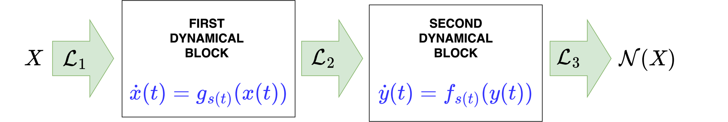
Neural networks motivated by dynamical systems

\( \mathcal{N}(x) = f_{\theta_L}\circ ... \circ f_{\theta_1}(x)\)

Neural networks motivated by dynamical systems

\( \mathcal{N}(x) = f_{\theta_L}\circ ... \circ f_{\theta_1}(x)\)

\mathcal{N}(x) = \Psi_{F_L}^{h_L}\circ ...\circ \Psi_{F_1}^{h_1}(x)

\( \dot{x}(t) = F(x(t),\theta(t))=:F_{s(t)}(x(t)) \)

Where \(F_i(x) = F(x,\theta_i)\)

\( \theta(t)\equiv \theta_i,\,\,t\in [t_i,t_{i+1}),\,\, h_i = t_{i}-t_{i-1}\)

t_0

t_1

t_2

t_i

t_{i+1}

t_L

\cdots

Neural networks motivated by dynamical systems

\dot{x}(t) = B(t)\mathrm{tanh}(A(t)x(t) + b(t))

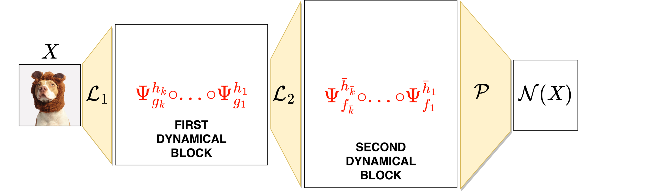
Neural networks motivated by dynamical systems

Accuracy is not all you need

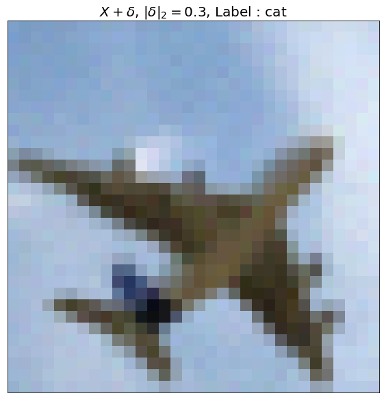
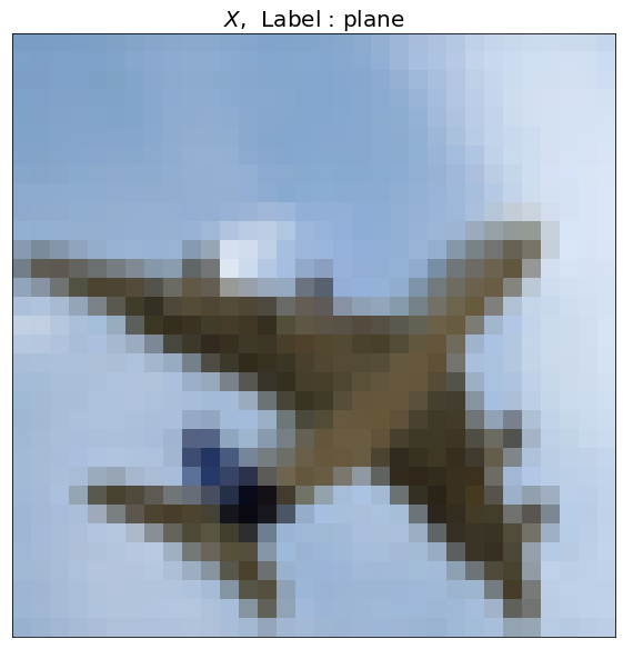
\(X\) , Label : Plane

\(X+\delta\), \(\|\delta\|_2=0.3\) , Label : Cat

GENERAL IDEA

EXAMPLE

Property \(\mathcal{P}\)

\(\mathcal{P}=\) Volume preservation

Imposing some structure

GENERAL IDEA

EXAMPLE

Property \(\mathcal{P}\)

\(\mathcal{P}=\) Volume preservation

Family \(\mathcal{F}\) of vector fields that satisfy \(\mathcal{P}\)

\(F_{\theta}(x,v) = \begin{bmatrix} \Sigma(Av+a) \\ \Sigma(Bx+b) \end{bmatrix} \)

\(\mathcal{F}=\{F_{\theta}:\,\,\theta\in\mathcal{P}\}\)

Imposing some structure

GENERAL IDEA

EXAMPLE

Property \(\mathcal{P}\)

\(\mathcal{P}=\) Volume preservation

Family \(\mathcal{F}\) of vector fields that satisfy \(\mathcal{P}\)

\(F_{\theta}(x,v) = \begin{bmatrix} \Sigma(Av+a) \\ \Sigma(Bx+b) \end{bmatrix} \)

\(\mathcal{F}=\{F_{\theta}:\,\,\theta\in\mathcal{P}\}\)

Integrator \(\Psi^h\) that preserves \(\mathcal{P}\)

x_{n+1}=x_n+h\Sigma(A_nv_n+a_n)\\ v_{n+1}=v_n+h\Sigma(B_nx_{n+1}+b_n)

Imposing some structure

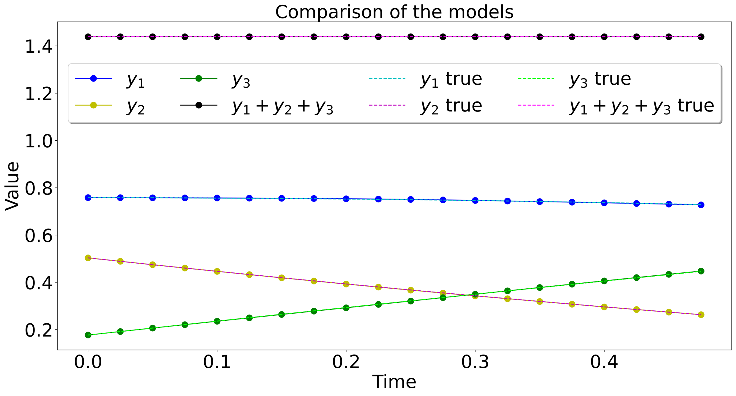
\dot{y} = \begin{bmatrix} 0 & -y_3y_1^2 & y_2y_3 \\ y_3y_1^2 & 0 & -\sin{y_1} \\ -y_2y_3 & \sin{y_1} & 0\end{bmatrix}\boldsymbol{1}

\dot{x}(t) = \{A_{\theta}(x(t))-A_{\theta}(x(t))^T\}\boldsymbol{1}\\ \mathrm{vec}(A_{\theta}(x)) = V\Sigma(Ux+u)\\ \theta=(U,V,u)

Mass-preserving networks

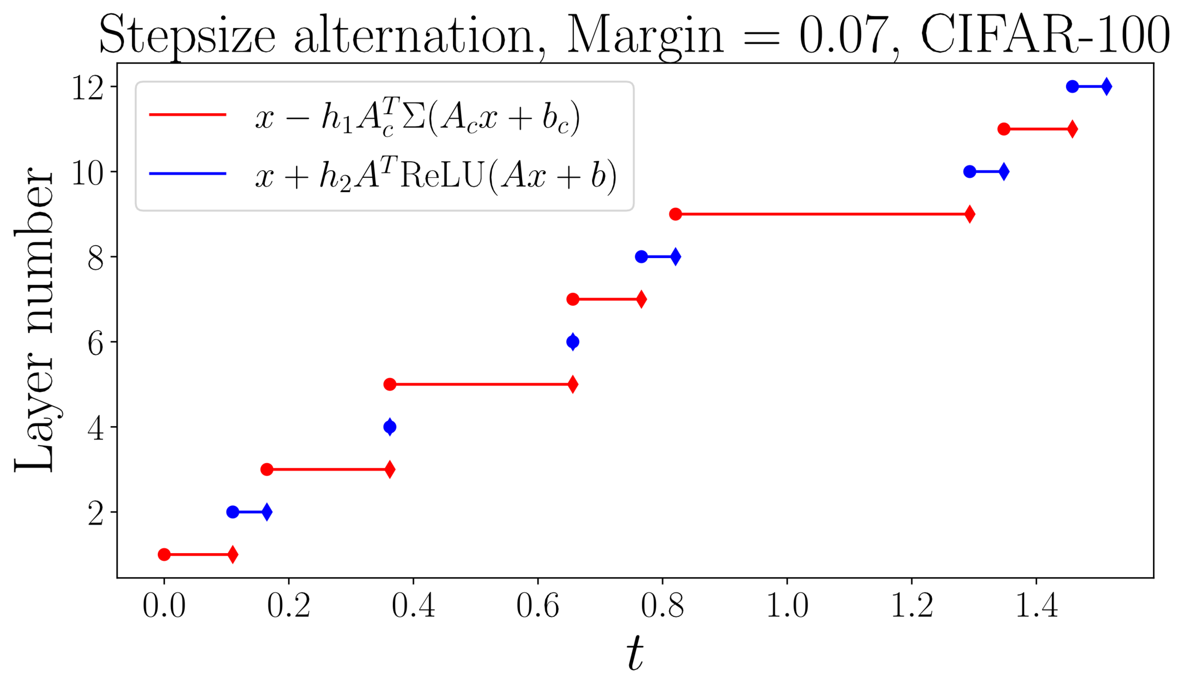
Lipschitz-constrained networks

\(m=1\)

\(m=\frac{1}{2}\)

\(\Sigma(x) = \max\left\{x,\frac{x}{2}\right\}\)

A_c^TA_c = A^TA = I

X_{\theta_i}(x) := - \nabla V_{\theta_i}(x) = -A_c^T\Sigma(A_cx+b_c)

\Psi^{h^i_C}_{X_{\theta_i}}(x) = x - h_cA_c^T\Sigma(A_cx+b_c)

Y_{\theta_i}(x) := A^T\mathrm{ReLU}(Ax + b)

\|\Psi^{h_c}_{X_{\theta_i}}(y) - \Psi^{h_c}_{X_{\theta_i}}(x)\|\leq \sqrt{1-{h_c}+h_c^2}\|y-x\|

\Psi^{h_e}_{Y_{\theta_i}}(x) = x + {h_e}A^T\mathrm{ReLU}(Ax+b)

\|\Psi^{h_e}_{Y_{\theta_i}}(y) - \Psi^{h_e}_{Y_{\theta_i}}(x)\|\leq (1+{h_e})\|y-x\|

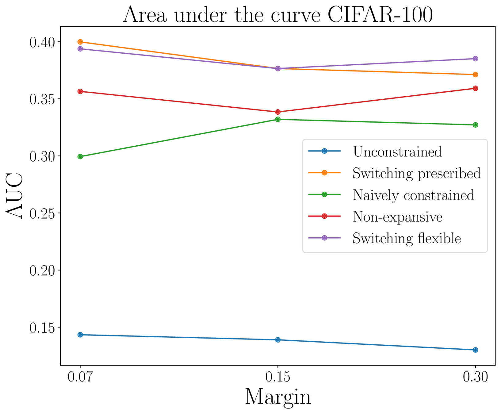
Lipschitz-constrained networks

\mathcal{N}_{\theta}(x)=\Psi_{X_{\theta_{2k}}}^{h_{2k}} \circ \Psi_{Y_{\theta_{2k-1}}}^{h_{2k-1}} \circ ... \circ \Psi_{X_{\theta_2}}^{h_2} \circ \Psi_{Y_{\theta_{1}}}^{h_1}(x)

\sqrt{1-{h_{2k}}+h_{2k}^2}(1+h_{2k-1})\leq 1

Lipschitz-constrained networks

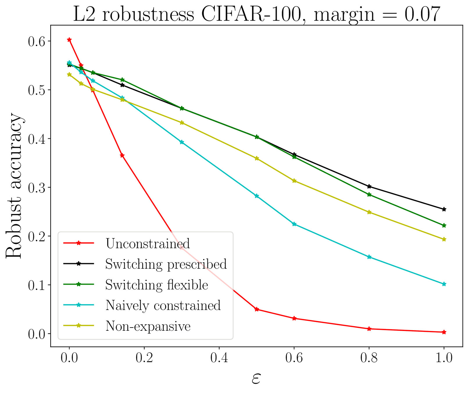
Adversarial robustness

Thank you for the attention

Celledoni, E., Murari, D., Owren B., Schönlieb C.B., Sherry F, preprint (2022). Dynamical systems' based neural networks

\(\texttt{davide.murari@ntnu.no}\)

Examples

\dot{x}(t) = -A^T(t)\Sigma(A(t)x(t) + b(t)) =\\ -\nabla \left( \boldsymbol{1}^T\Gamma(A(t)x(t)+b(t)) \right)

\dot{x}(t) = \mathbb{J}A^T(t)\Sigma(A(t)x(t)+b(t))

\ddot{x}(t) = \Sigma(A(t)x(t)+b(t))

1-LIPSCHITZ NETWORKS

HAMILTONIAN NETWORKS

VOLUME PRESERVING, INVERTIBLE

Naively constrained networks

x\mapsto F_{\theta_i}(x):=\frac{1}{2}\left(x + A_i\Sigma(B_ix+b_i)\right)\\ \|A_i\|_2,\|B_i\|_2\leq 1\\ \mathcal{N}_{\theta}(x) = F_{\theta_L}\circ ... \circ F_{\theta_1}(x)